

- EAER>
- Journal Archive>
- Contents>
- articleView
Contents
Citation
| No | Title |
|---|---|
| 1 | The gravity model and trade in intermediate inputs / 2020 / The World Economy / vol.43, no.8, pp.2034 / |
Article View
East Asian Economic Review Vol. 21, No. 4, 2017. pp. 295-315.
DOI https://dx.doi.org/10.11644/KIEP.EAER.2017.21.4.332
Number of citation : 1View
667
Download
375
Gravity with Intermediate Goods Trade
|
|
Metro Seoul |
|---|---|
|
|
Sogang University |

Abstract
This paper derives the gravity equation with intermediate goods trade. We extend a standard monopolistic competition model to incorporate intermediate goods trade, and show that the gravity equation with intermediates trade is identical to the one without it except in that gross output should be used as the output measure instead of value added. We also show that the output elasticity of trade is significantly underestimated when value added is used as the output measure. This implies that with the conventional gravity equation, the contribution of output growth can be substantially underestimated and the role of trade costs reduction can be exaggerated in explaining trade expansion, as we demonstrate for the case of Korea’s trade growth between 1995 and 2007.
JEL Classification: F12, F14, F15
Keywords
Gravity Equation, Gross Output, Intermediate Goods Trade, Global Value Chains, Fragmentation
I. INTRODUCTION
Last several decades saw a huge increase in the trade of intermediate goods across countries. This phenomenon was driven by the rise of global supply chains, also called by various other names, such as fragmentation, unbundling, or vertical specialization of production. A production process is broken into a number of parts, which then are relocated in various countries of the world. As a result, unfinished products cross borders multiple times before they reach a final user, and trade volume increases relative to value added produced by trade.
The new aspect of world trade can be understood by investigating world input-output tables or analyzing a computable general equilibrium model embodying worldwide input-output structure. Hummels, Ishii and Yi (2001), Yi (2003), Johnson and Noguera (2012), Bridgman (2012), and Koopman, Wang and Wei (2014) are notable examples in this line of research.
An alternative approach is to modify the gravity equation to encompass intermediate goods trade. The gravity equation states that bilateral trade is proportional to the product of the masses of trading pairs, and is inversely related to trade costs between them. It has been the most powerful and popular tool for estimating the determinants of bilateral trade flows. The gravity model gained more traction in recent years since Eaton and Kortum (2002), Anderson and van Wincoop (2003), and Chaney (2008) strengthened its theoretical foundation by rigorously deriving it from muti-country Ricardian, Chamberlinian, and heterogeneous firms trade models.
Modifying the gravity equation to incorporate intermediates trade should start from a simple observation that trade is measured in gross sales, while GDP is measured in value added. Most theoretical studies on the gravity equation assume the world without intermediates goods, and thus ignore the difference between gross sales and value added. Most empirical studies estimating the gravity equation use GDP to measure the mass of a country, either because trade theories ignoring the presence of intermediate goods justify its use, or because data on gross output are not easily available. However, one can conjecture that to obtain reliable results, either trade in terms of value added should be regressed on value added output, or trade in gross sales should be regressed on gross output. The former approach, as exemplified by Aichele and Heiland (2014), would require a complicated task of collapsing the inverse matrix coefficients of input-output tables into a manageable number of explanatory variables. Reduced gravity equations would be model-specific or their coefficients would be difficult to link to structural parameters.
In this paper, we take the latter approach of explaining gross trade by gross output. A number of researchers have estimated the gravity equation by regressing gross trade on gross output because it made more intuitive sense (e.g., Wei, 1996 and Novy, 2013). However, they do not offer any theoretical justification. The paper by Baldwin and Taglioni (2011), to our knowledge, is the first study that formally derives the gravity equation with intermediate goods trade, and emphasizes the importance of using gross output as the mass variable. We build upon their results, and show that the mass variable of the gravity equation with intermediated goods trade should be gross output for the exporter, and gross output plus net imports for the importer.1 We derive this result in a general setting where the ratio of value added to gross output responds to economic variables such that using value added as the mass variable generates errors-in-variables bias. Most trade models with intermediate goods (e.g., Krugman and Venables, 1996; Eaton and Kortum, 2002; Baldwin and Taglioni, 2011) assume that the production function for gross output is of Cobb-Douglas, and thus the ratio of value added to gross output is fixed. Under this assumption, value added is a perfect proxy for gross output, and the question that we raise in this paper becomes meaningless.
A convenient feature of our gravity equation is that it holds both for aggregate trade and for sectoral level trade. A number of empirical studies on gravity estimate the gravity equation at sectoral level. Some studies aim to demonstrate that the elasticity of trade with respect to output, trade costs, or exchange rate volatility varies depending on the nature of goods, while others try to capture a trade pattern specific to an industry. Rauch (1999), Feenstra et al. (2001), Evans (2003), Saito (2004), Baldwin et al. (2005), and Anderson et al. (2014) are just a few such examples. In this line of research, it has never been entirely clear which mass variable should be used for the exporter and which for the importer. This paper provides a rigorous answer to this question.
In addition, this paper tests whether the use of gross output as the mass variable improves the performance of the gravity equation over the popular practice of using value added as the mass variable. Baldwin and Taglioni (2011) also conduct a similar comparison. Because data on gross output are not widely available, they suggest using the sum of GDP and intermediate goods trade as a proxy, and show that the proxy performs better than GDP in gravity equation estimations. In this paper, we use gross output data from the World Input-Output Table (Timmer et al., 2015), and explicitly show that fluctuations in gross output to value added ratio generate downward bias in the estimation of the mass variable coefficient when value added is used as the mass variable. This implies that if we use the conventional gravity equation with value added as the mass variable, the contribution of output growth can be substantially underestimated, and the role of trade costs reduction can be significantly exaggerated in explaining trade expansion. We demonstrate this possibility using the case of Korea’s trade growth between 1995 and 2007.
This paper is organized as follows. In section II, we derive the gravity equation in the presence of intermediate goods trade from a monopolistic competition model with intermediate goods trade. In section III, we estimate the gravity equation, and compare the empirical performance of value added and gross output as the mass variable. Section III briefly concludes this paper.
1)
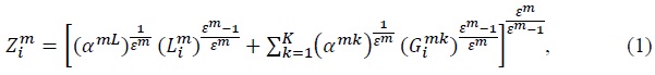
II. THEORY
To introduce intermediate goods trade into the gravity theory, we utilize the framework used by Krugman and Venables (1996), Eaton and Kortum (2002), and Baldwin and Taglioni (2011). The essence of the idea is the assumption that each firm produces a good (or a service) that can be used both as an intermediate good and as a final good. We incorporate the idea into the monopolistic competition model by Krugman (1979) and Anderson and van Wincoop (2003), where all firms located in the same country are assumed to be symmetrical.
There are  be its measure. Free entry prevails everywhere and the profit of each firm is equal to zero.
To produce  units of
  are required.
  is the fixed cost of production, and
  is the marginal cost, both measured in the unit of
  is a composite good, which is produced by a CES production function using local labor
  and composite intermediate goods
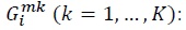
 intermediate good
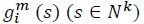 is the input of an industry
  is the elasticity of substitution between
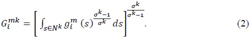
  and is greater than one. We assume that individual goods entering composite intermediate goods are tradable, but composite goods themselves are not tradable. Equation (2) implicitly assumes that
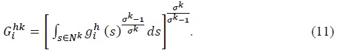
The unit cost of  is given by the following price index:

 can be written as:

Thus the total cost of a country

Denoting the marginal cost by 

Applying Shephard’s lemma to (4), we can obtain the shares of labor and composite intermediate goods in the total cost of a country
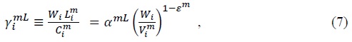
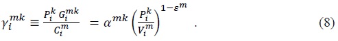
Using (3), (4), and (8), we can derive the value of good
The representative household in country
Here, superscript  is composite good
Composite final good
Using the same method as before, we can show that
 is the share of composite good
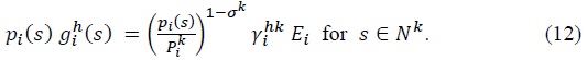
To maximize the profit, a firm sets its price as a markup over the marginal cost, the markup rate determined by the price elasticity of its demand. By CES demand functions given in (9) and (12), the price elasticity for an industry
 is the price of an industry
  represents an iceberg-type transportation cost, and a firm in country
  units of a good to sell one unit in country
 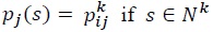 and
and
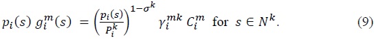
By (9)and (12), the value of good
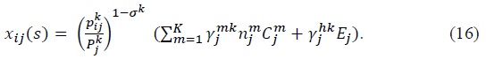
Equation (16) is crucial for our result below. The essential feature of the equation that allows the gravity equation to follow from it is that demand for good 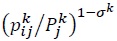 and total expenditure on good
 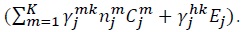 This property, in turn, follows from our assumption that composite input
The rest of derivation is straightforward. Because
From the assumption that the profit of each firm is zero, the total costs incurred by industry  is equal to the gross output of industry
  Then we can show that:

Equation (18) is an accounting identity that holds in any input-output model: the total value of industry  plus their imports
  minus their exports
  To see this more formally, we divide
  into two parts: the share of domestically produced goods
  and the share of imported goods
The last equality follows from the fact that 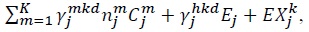 which is equal to the home sales of domestically produced industry
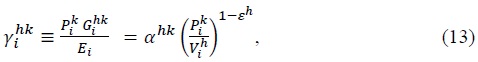
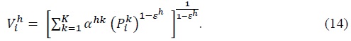
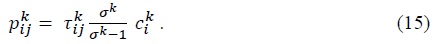
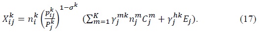
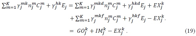
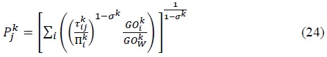
Using (15) and (18), we rewrite (17) as
where 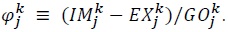 The summation of
  over all
  must be equal to the gross output of industry
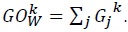 Define
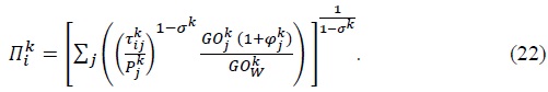
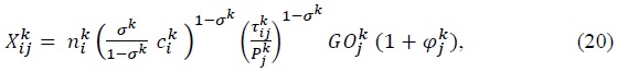
Solving for 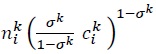 in (21), and plugging the solution into (20) together with (22) yields the gravity equation for a world with intermediate goods trade.
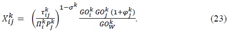
Using (3), (15), and (21), we can show that
Equation (23) states that exports from country 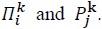 Equation (23) is essentially identical to the gravity equation derived by Anderson and van Wincoop (2003). The only difference is that here we are dealing with sectoral level trade covering both final goods and intermediate goods, and we use gross output to measure the mass of a country, not GDP.2
Equation (23) implies that using value-added as the mass variable is permissible to the extent that value-added is proportional to gross output. However, the ratio of value added to gross output given in (7)  will change whenever the intermediate good price index changes relative to the wage rate, unless the elasticity of substitution between labor and intermediate goods is equal to 1. With a non-unitary elasticity of substitution, the ratio will fluctuate whenever raw material prices, trade barriers or the number of intermediate goods change.
The equation that we will estimate comes from the logarithmic version of (23).
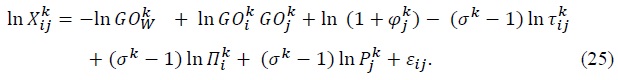
Time subscripts are dropped for notational simplicity. As is standard in the literature, we assume that bilateral transportation costs are determined by the following equation.
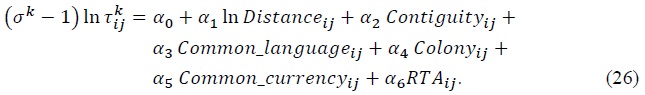
 by year fixed effects. As has now become standard, the effects of multilateral resistance variables
  respectively, are estimated by exporter fixed effects and importer fixed effects.3 Thus, our benchmark estimation equation is given by:
2)Another minor difference is that we adjust for trade imbalance.
3)Because multilateral resistance can change over time, we should, in principle, allow country fixed effects to vary over years. However, this necessitates plugging more than 1,000 dummy variables in the equation, and causes a collinearity problem with the mass variable ln  and other dummies. Thus we allow for only time-invariant exporter and importer fixed effects
III. SOME EMPIRICAL RESULTS
In this section, we test whether using gross output as the mass variable improves the empirical performance of the gravity equation. Our data come from the following sources. For bilateral trade, gross output, and value added, we use annual data from the World Input-Output Database Release 2013 (Timmer et al., 2015). The database provides annual data for 40 countries and 1560 (=40×39) country pairs, which include most major industrial countries and some emerging economies. Some data in the database are estimated rather than observed, but the database has the big advantage of providing the three interconnected variables in a mutually consistent way. Data for distance and the dummy variables come from the CEPII gravity dataset (Head, Mayer, and Ries, 2010; Head and Mayer, 2014). We will restrict our analysis to trade in manufacturing (industry 3 through industry 16). We take this choice because the manufacture sector took center stage in the rise of global value chains, and in the resulting increase in the ratio of gross output to value added during the last two decades. The period of examination is 13 years from 1995 through 2007. Note that this is the period when world trade as a share of GDP increased at a record speed with the rapid expansion of global value chains.4
Estimation results using pooled OLS estimation are reported in Table 1. The main concern of Baldwin and Taglioni (2011) is that in the presence of intermediates trade, the conventional method of employing value added as the mass variable has the danger of generating bias in estimating the output elasticity of trade. They show that this bias reduces the estimated coefficient of the mass variable toward zero, more so for trade flows between country pairs doing massive intermediates trade. To check if this problem also shows up in our dataset, in regression (1), we use value added as the mass variable as in standard gravity equations. The coefficient of ln
In Table 2, we report estimation results when exporter and importer fixed effects are replaced by exporter-importer pair fixed effects. This exercise is for the possibility that explanatory variables that we placed to control for bilateral trade costs still omit some important variables affecting bilateral trade costs, and generate significant bias. In addition, for many policy questions, the response of trade over time is more relevant than that across countries. In Table 2, we can see that the coefficients of the mass variables change surprisingly little with country pair fixed effects, even though the coefficients for
As we emphasized before, our gravity equation holds both for aggregate trade and for industry level trade. Relying on this feature, we estimated gravity equations for 14 manufacturing industries. Regression results vary a lot from industry to industry. However, in almost all industries, using valued added alone as the mass variable results in the underestimation of its coefficient, and using gross output instead significantly raises the estimated coefficient. In addition, in all industries, the estimated coefficient of ln (
Table 3 reports results for three selected industries. To save space, the results when ln
The question that we are pursuing here is whether we should use value added or gross output to correctly estimate the elasticity of trade with respect to output. The literature on the gravity equation, however, has moved away from the issue. The gravity equation is mainly used as a tool for evaluating the effect on trade volume of shocks reducing trade barriers, such as free trade agreements, currency unions, or lower transportation costs. Therefore, researchers’ interests converged on correctly estimating the elasticities of trade with respect to trade frictions. These elasticities can be consistently estimated in the gravity equation without specifying the mass variable. Instead of using ln
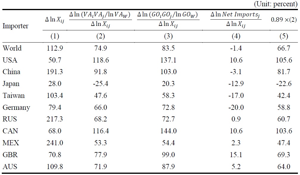
To get a sense on how important the correct specification of the mass variable is in decomposing trade expansion, we construct Table 4. Column (1) shows the growth of Korea’s manufactured exports to the world and its top 10 importers between 1995 and 2007. Columns (2) and (3), respectively, display the ratio of percentage increase in value added to percentage increase in exports, and the ratio of percentage increase in gross output to percentage increase in exports. Column (4) shows the ratio of percentage increase in importer’s net imports to percentage increase in exports. The numbers in the third row, which accounts for Korea’s exports to the world, are obtained by calculating the weighted averages of the numbers corresponding to individual countries, each weight given by the average share of an importer in Korea’s total exports during the period.6 The row shows that Korea’s manufactured exports grew 113% during the period, and 75% of the growth can be attributed to the growth of valued added produced by Korea and its trading partners. The number increases to 84% when gross output is used instead of value added as the output variable. This is because the ratio of gross output to value added increased in Korea and other countries. Column (4) shows that the part explained by importer’s net imports is small at -1.4%. The following rows report results for individual countries. They vary a lot from country to country. However, we can notice that for all countries, the part explained by gross output is larger than that by valued added. The part explained by importer’s net imports is large in some countries.
Column (5) was obtained by multiplying 0.89, the estimated coefficient of ln
4)The database covers the period from 1995 through 2011. However, China’s gross output to value added ratio, which is a key variable for our investigation, is fixed to a constant number during the period between 2008 and 2011, casting doubt on the quality of data during this period. We also want to avoid the period of trade turmoil after the Great Financial Crisis of 2008. However, our main results do not depend on dropping the period.
5)Correctly estimating the output elasticity of trade is also important in understanding the recent slowdown of world trade relative to GDP growth. See
6)The World Input-Output Database provides Korea’s exports to 39 other countries and the rest of the world. The rest of the world accounts for 26 percent of Korea’s total exports.
IV. CONCLUSION
In this paper, we propose a simple solution to the problem of estimating the gravity equation in the presence of intermediate goods trade. All we have to do is to use gross output in place of value added as the mass variable. This method can reduce bias coming from fluctuations in gross output to value added ratio, which would naturally arise in the world where intermediate goods are heavily traded through global supply networks.
Through some empirical exercises, we show that bias is not quite large, but significant for the gravity equation in manufacturing trade. However, huge bias can arise for an industry level gravity equation, as we demonstrate in the case of petroleum refining industry. We also show that this bias can result in exaggerating the role of reduced trade barriers in explaining the recent expansion of world trade. In the case of Korea’s export growth between 1995 and 2007, the possible contribution of reduced trade barriers shrinks from 33% to 16% of Korea’s total export growth. This suggests that the effect of trade policy changes like the Korea-US FTA or the Korea-EU FTA could be substantially overestimated with the conventional gravity equation using GDP as the mass variable.
One limitation of our study is that our empirics focused only on the period in which world trade rapidly expanded with the rise of global value chains. It will be an interesting exercise to test whether our findings are still valid for the period after 2011, in which world trade shrank relative to GDP. However, the new release of the World Input-Output Database contains only a few observations on the period, and observations for the recent years in which world trade shrank most, are not feasible yet. Thus, we leave it to our future investigations.
Finally, we would like to mention that the approach of this paper can trace only one face of global value chains through the ratio of gross output to value added. Thus, it has a serious limitation as a portrait of changing global production networks. Its usefulness should be found as a simple way of supplementing other methods of investigating world trade structure.
Tables & Figures
Table 1.
Value Added Vs. Gross Output in the Gravity Equation
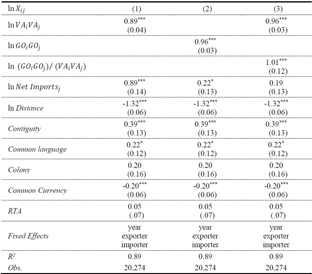
Note: The intercepts are not reported. The numbers in the parentheses are robust standard errors clustered by country-pairs.
Table 2.
Value Added Vs. Gross Output in the Gravity Equation: Panel Estimation
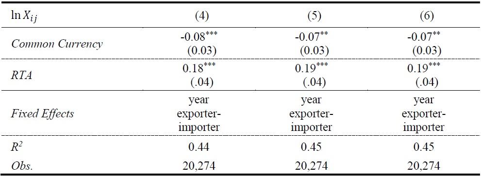
Table 2.
Continued

Note: Some bilateral costs variables in Tables 1 and 2 are dropped because they are constant over time. The intercepts are not reported. The numbers in the parentheses are robust standard errors clustered by country-pairs.
Table 3.
Value Added Vs. Gross Output in the Gravity Equation in Selected Industries
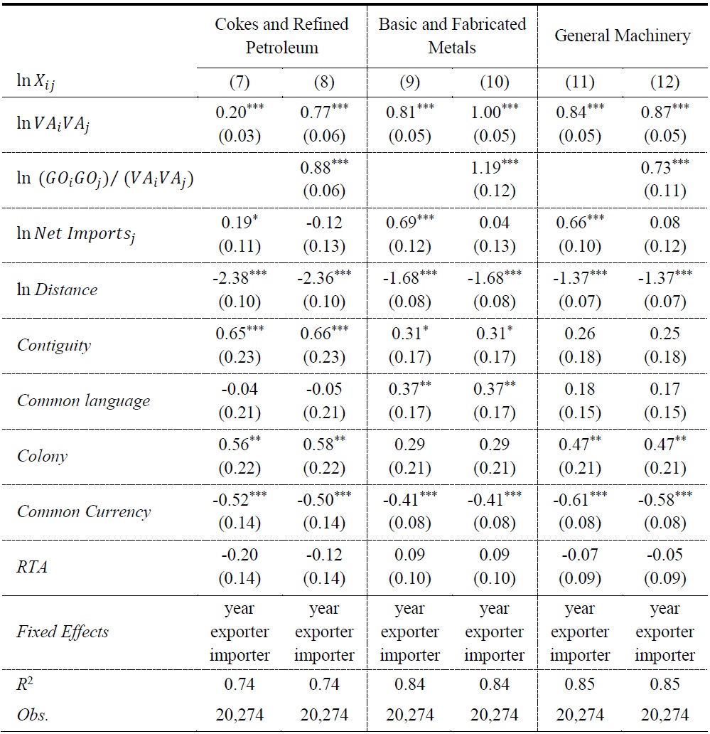
Note: The intercepts are not reported. The numbers in the parentheses are robust standard errors clustered by country-pairs.
Table 4.
Decomposing Korea’s Manufacturing Export Growth Between 1995 and 2007
References
- Aichele, R. and I. Heiland. 2014. “Where is the Value Added? China’s WTO Entry, Trade and Value Chains,” In Beiträge zur Jahrestagung des Vereins für Socialpolitik 2014: Evidenzbasierte irtschaftspolitik-Session: China’s Growing Role in World Trade, no. E12-V3.
-
Anderson, J. E., Milot, C. A. and Y. V. Yotov. 2014. “How Much Does Geography Deflect Services Trade? Canadian Answers,”
International Economic Review , vol. 55, no. 3, pp. 791-818.
-
Anderson, J. E. and E. van Wincoop. 2003. “Gravity with Gravitas: A Solution to the Border Puzzle,”
American Economic Review , vol. 93, no. 1, pp. 170-192.
-
Baier, S. L. and J. H. Bergstrand. 2001. “The Growth of World Trade: Tariffs, Transportation Costs, and Income Similarity,”
Journal of International Economics , vol. 53, no. 1, pp. 1-27.
- Baldwin, R. E., Skudelny, F. and D. Taglioni. 2005. “Trade Effects of the Euro: Evidence from Sectoral Data,” ECB Working Paper, no. 446.
- Baldwin, R. and D. Taglioni. 2011. “Gravity Chains: Estimating Bilateral Trade Flows When Parts and Components Trade is Important,” NBER Working Paper, no. 16672.
-
Bridgman, B. 2012. “The Rise of Vertical Specialization Trade,”
Journal of International Economics , vol. 86, no. 1, pp. 133-140.
- Constantinescu, C., Mattoo, A. and M. Ruta. 2015. “The Global Trade Slowdown: Cyclical or Structural?,” IMF Working Paper, no. 15/6.
-
Chaney, T. 2008. “Distorted Gravity: The Intensive and Extensive Margins of International Trade,”
American Economic Review , vol. 98, no. 4, pp. 1707-1721.
-
Eaton, J. and S. Kortum. 2002. “Technology, Geography, and Trade,”
Econometrica , vol. 70, no. 5, pp. 1741-1779.
-
Estevadeordal, A., Frantz, B. and A. M. Taylor. 2003. “The Rise and Fall of World Trade, 1870-1939,”
Quarterly Journal of Economics , vol. 118, no. 2, pp. 359-407.
-
Evans, C. L. 2003. “The Economic Significance of National Border Effects,”
American Economic Review , vol. 93, no. 4, pp. 1291-1312.
-
Feenstra, R. C., Markusen, J. A. and A. K. Rose. 2001. “Using the Gravity Equation to Differentiate among the Alternative Theories of Trade,”
Canadian Journal of Economics , vol. 34, no. 2, pp. 430-447.
-
Head, K., Mayer, T. and J. Ries. 2010. “The Erosion of Colonial Trade Linkages after Independence,”
Journal of International Economics , vol. 81, no. 1, pp. 1-14.
-
Head, K. and T. Mayer. 2014. Gravity Equations: Workhorse, Toolkit, and Cookbook. In Gopinath, G., Helpman E. and K. Rogoff. (eds.)
Handbook of International Economics , vol. 4. Amsterdam: Elsevier. -
Hummels, D., Ishii, J. and K.-M. Yi. 2001. “The Nature and Growth of Vertical Specialization in World Trade,”
Journal of International Economics , vol. 54, no. 1, pp. 75-96.
- Jang, S. 2014. “Vertical Specialization and Gravity Equation Estimation,” Master Thesis, Sogang University.
-
Johnson, R. C. and G. Noguera. 2012. “Accounting for Intermediates: Production Sharing and Trade in Value Added,”
Journal of International Economics , vol. 86, no. 2, pp. 224-236.
-
Koopman, R., Wang, Z. and S-J. Wei. 2014. “Tracing Value-Added and Double Counting in Gross Exports,”
American Economic Review , vol. 104, no. 2, pp. 459-494.
-
Krugman, P. R. 1979. “Increasing Returns, Monopolistic Competition, and International Trade,”
Journal of International Economics , vol. 9, no. 4, pp. 469-479.
-
Krugman, P. and A. J. Venables. 1996. “Integration, Specialization, and Adjustment,”
European Economic Review , vol. 40, no. 3-5, pp. 959-967.
-
Novy, D. 2013. “Gravity Redux: Measuring International Trade Costs with Panel Data,”
Economic Inquiry , vol. 51, no. 1, pp. 101-121.
-
Rauch, J. E. 1999. “Networks versus Markets in International Trade,”
Journal of International Economics , vol. 48, no. 1, pp. 7-37.
-
Saito, M. 2004. “Armington Elasticities in Intermediate Inputs Trade: A Problem in Using Multilateral Trade Data,”
Canadian Journal of Economics , vol. 37, no. 4, pp. 1097-1117.
-
Timmer, M. P., Dietzenbacher, E., Los, B., Stehrer, R. and G. J. de Vries. 2015. “An Illustrated User Guide to the World Input–Output Database: The Case of Global Automotive Production,”
Review of International Economics , vol. 23, no. 3, pp. 575-605.
- Wei, S.-J. 1996. “Intra-National versus International Trade: How Stubborn are Nations in Global Integration?,” NBER Working Paper, no. 5531.
-
Yi, K.-M. 2003. “Can Vertical Specialization Explain the Growth of World Trade?,”
Journal of Political Economy , vol. 111, no. 1, pp. 52-102.