

- EAER>
- Journal Archive>
- Contents>
- articleView
Contents
Citation
| No | Title |
|---|---|
| 1 | The Key Success Factors for Attracting Foreign Investment in the Post-Epidemic Era / 2021 / Axioms / vol.10, no.3, pp.140 / |
| 2 | Does R&D investment moderate the relationship between the COVID-19 pandemic and firm performance in China’s high-tech industries? Based on DuPont components / 2022 / Technology Analysis & Strategic Management / vol.34, no.12, pp.1464 / |
| 3 | / 2022 / pp.247 / |
| 4 | GVCs in times of global crises and economic regionalization: Case of Russian oil and gas industry / 2023 / E3S Web of Conferences / vol.460, pp.02014 / |
Article View
East Asian Economic Review Vol. 24, No. 4, 2020. pp. 389-416.
DOI https://dx.doi.org/10.11644/KIEP.EAER.2020.24.4.385
Number of citation : 4View
106
Download
97
The Reorganization of Global Value Chains in East Asia before and after COVID-19
|
|
OECD |
|---|

Abstract
This paper provides empirical evidence on the reorganization of GVCs in East Asia, highlighting that structural trends explain a decrease in the fragmentation of production after 2011 but that it is not the result of rising trade costs along the value chain. Using harmonized inter-country input-output tables, the paper first analyzes the global import intensity of production to document changes in the structure of GVCs. It then calculates theory-consistent bilateral trade costs for intermediate and final products using an approach derived from the gravity literature and introduces a new index of cumulative trade costs along the value chain. These data are used to discuss whether the decrease in global imports is the consequence of shifts in demand, efficiency-enhancing strategies of firms or rising trade costs. Between 2011 and 2016, cumulative trade costs have decreased in East Asian GVCs. However, as COVID-19 is likely to intensify trade and investment uncertainties, trade costs could increase in the future. Policies aimed at reducing uncertainties and preserving the gains from trade and investment liberalization will be key in this new environment.
JEL Classification: F14, F60, L16
Keywords
Global Value Chain, Import Intensity, Fragmentation of Production, Trade Costs, Input-Output
I. INTRODUCTION
Many studies have described the rise of global value chains (GVCs) and the opportunities they have provided for countries to integrate into the world economy and generate more income (OECD, 2013; Baldwin, 2016; Taglioni and Winkler, 2016; World Bank, 2019). GVCs have played an important role in East Asia where they are associated with export-led growth strategies and the emergence of ‘factory Asia’ (Baldwin and Forslid, 2014).
However, since the Great Financial Crisis, there has been a stagnation or even a decline in the international fragmentation of production (Miroudot and Nordström, 2020). An important question is whether this decline is explained by structural trends related to technology (e.g. the spread of digital technologies and advanced robotics) or changes in the preferences of consumers (e.g. more socially and environmentally responsible consumption), as opposed to rising trade costs in the context of trade tensions and the decoupling of the US economy from China. In addition, COVID-19 has triggered a new debate on the future of GVCs in relation to the vulnerabilities of international supply chains (Miroudot, 2020).
This paper reviews evidence on structural changes in GVCs in East Asia since 2011 and discusses the impact of COVID-19. There are no data yet that can allow us to describe the post-COVID world but many of the changes that are currently under way in GVCs have started before the pandemic and a closer look at existing trends gives insights on what we can expect.
The development of inter-country input-output (ICIO) tables offers new empirical tools to understand GVCs (Timmer et al., 2014 and 2016; Johnson, 2018; Miroudot and Ye, 2020). Using input-output techniques, one can decompose output and trade flows to identify the contribution of all countries and industries in the value chain. Moreover, the combination of data on intermediate and final products allows to disentangle structural changes in GVCs from changes related to shifts in final demand. While these tools are useful to analyze GVCs, they do not provide an explanation for the underlying drivers of the transformation of supply chains. In particular, it is difficult to isolate the impact of trade costs and their policy component (e.g. new tariffs) from changes in other costs or consumers’ preferences.
As there is also a growing literature on the estimation of trade costs (Anderson and Yotov, 2010; Novy, 2013; Anderson et al., 2018), this paper combines input-output techniques with the calculation of bilateral trade costs in order to provide quantitative evidence on the evolution of trade costs along the value chain. A new index of cumulative trade costs is calculated to check whether rising trade tensions and more protectionist policies are among the drivers of the recent ‘de-globalization’.
The question is especially important for East Asia as it includes the Chinese economy and countries such as Korea and Japan that are both integrated in trade and production networks with the US and China. While there is a ‘new normal’ in the global trading system that affects East Asia (Choi, 2020), it is not clear that the region will follow the path of protectionism and economic nationalism in the post-COVID world. There are also data that suggest that the decrease in the fragmentation of production might be more limited in East Asia and that GVCs are still expanding (Obashi and Kimura, 2018). This is why a focus on this region is relevant.
Against this backdrop, the rest of the paper is organized as follows. Section II describes the data used in the paper and the methodology followed to look at imports along the value chain and to calculate cumulative trade costs along the value chain. Section III gives an overview of the main trends in GVCs in East Asia relying on the global import intensity and a decomposition of global imports. Section IV analyzes the evolution of trade costs along the value chain and the role they have played in the reorganization of GVCs. Section V discusses the impact of COVID-19 and the way firms adjust to risks and policy uncertainties. Section VI concludes.
II. METHODOLOGY AND DATA
The empirical analysis in this paper relies on the OECD ICIO tables released in December 2018. These tables include information on production and trade in 64 economies (plus a ‘rest of the world’) and 36 industrial sectors in the ISIC Rev. 4 classification. The period covered is 2005-2016. All inter-country inter-industry transactions are included in a matrix of intermediate consumption and a matrix of final demand, allowing the use of input-output techniques to derive indicators of the fragmentation of production. For China and Mexico, data are heterogeneous and provide different input-output coefficients for firms engaged in international trade and firms focusing on domestic sales (i.e. China and Mexico are split into two ‘economies’).
1. Imports along the Value Chain
To study the fragmentation of production, an interesting indicator is the global import intensity (GII) introduced by Timmer et al. (2016). This indicator focuses on the imports needed to produce any type of good or service, whether exported or consumed in the domestic economy. It does not remove the double counting in imports and accounts for all trade flows related to production or final demand in a specific country and industry. GII is thus an indicator that not only reflects the foreign origin of inputs used in production but also the intensity of the fragmentation of production. The more production is fragmented across countries, the more the value of imported inputs is counted multiple times and the higher the value of GII.
Formally and using matrix notation, GII is calculated as follows. Let C be a matrix of intermediate consumption for G countries and N industries. It has the dimension GN x GN (which is 2,412 x 2,412 in the case of the OECD ICIO with 65 countries, 36 industries and heterogeneous data for China and Mexico).
To calculate all the imports needed along the value chain to produce one unit of final output in country

where  the transposition of the summation vector (i.e. a row vector of dimension GN with ones). The symbol ∘ is used to indicate an elementwise multiplication (i.e. Hadamard product) and the bar symbol refers to a diagonal matrix (i.e. vector [(
Once the GII indicator is calculated for all countries and industries in the dataset, values can be aggregated by using a final demand weighted average. Moreover, as demonstrated by Timmer et al. (2016), the value of GII for the world economy is simply equal to total imports of intermediate goods and services (across all countries and industries) divided by world GDP.
The analysis of trade in intermediate inputs can be complemented by a similar analysis for trade in final goods and services. Final demand in each country is also met by final products that are imported. Their value is directly known from the off-diagonal block elements of the  as the matrix of final demand expressed as a share of world GDP (which is equal to world final demand), world imports can be decomposed as:

where matrix and matrix that isolates cross-border transactions and removes domestic final demand.2
Furthermore, by replacing in equation (2) by  i.e. a matrix of dimension GNxG where the column of a specific country
2. Calculation of Bilateral Trade Costs
Being equipped with tools that allow us to account for all imports in the value chain, we are then interested in understanding the role of trade costs in explaining changes in the structure of GVCs. There are several approaches to calculate or estimate bilateral trade costs. The literature generally relies on the gravity model and methods aimed at recovering theory-consistent bilateral trade costs from trade data while eliminating country-specific structural characteristics (Head and Ries, 2001; Novy, 2013; Caliendo and Parro, 2015; Anderson et al., 2018).
Trade costs are derived from a comparison between theoretical trade flows in a frictionless world (based on theory) and actual trade flows (as measured in trade statistics). Different approaches are then available to disentangle partial equilibrium bilateral trade costs from country-specific general equilibrium structural terms and an error term related to noise in the data. Here, we rely on a calculation approach proposed by Novy (2013) that can easily be implemented using the OECD ICIO tables.
The starting point of this approach is the structural gravity model (Anderson and van Wincoop, 2003; Anderson and Yotov, 2010). Assuming identical preferences or technologies across countries (i.e. a globally common constant elasticity of substitution between products within each industry), the model explains bilateral trade at user prices as a function of expenditures in the importing country and sales in the exporting economy expressed as a share of world output (the frictionless value of trade) and a variable bilateral trade cost affected by trade costs with other partners (the distortion in trade induced by trade costs). It can be formally introduced through a system of equations, as below:
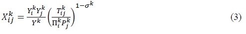
In equation (3),  is the value of shipments3 of product
  the sales of product
  the expenditures on product
  is a partial equilibrium bilateral trade cost between country
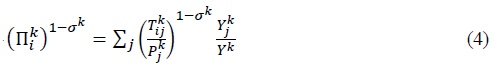
However, bilateral trade is also affected by trade costs with other partners, summarized in two multilateral resistance terms that account for general equilibrium effects:  in equation (4) is the outward multilateral resistance and aggregates the incidence of all bilateral trade costs borne by the producers of product
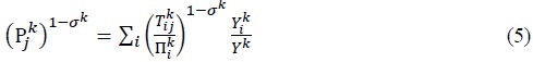
  in equation (5) is the inward multilateral resistance and accounts for the incidence of all bilateral trade costs on buyers of product
The strategy suggested by Novy (2013) builds on Head and Ries (2001) and consists of multiplying the structural gravity equation (8) describing trade flows from
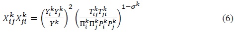
Writing equation (3) for  (i.e. intra-national trade) and substituting in equation (6) the product of outward and inward multilateral resistance terms for intra-national trade in
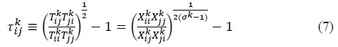
where  measures bilateral trade costs
  relative to domestic trade costs
  and is the geometric mean of barriers to trade in both directions. One is subtracted in order to obtain a tariff equivalent.
Multilateral resistance terms that are unobservable have disappeared in equation (7) and the only variables that are left are observed trade flows (including intra-national trade flows) and a parameter
 gives us the geometric mean between
 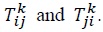 While it has the advantage of not capturing the impact of multilateral resistance, it does not indicate whether trade costs are when exporting from
  and general equilibrium trade costs related to multilateral resistance terms
  Agnosteva et al. (2014) describe such a ‘total trade costs’ index calculated as:

While it is unidirectional (i.e. it has a different value for  it does not distinguish the bilateral trade costs from multilateral resistance effects.
3. Trade Costs along the Value Chain
Once we have obtained bilateral trade costs for all country pairs and industries, the last step in the analysis consists in aggregating these trade costs along the value chain to obtain an index that reflects not only trade barriers between
Bilateral trade costs for final products are directly given by the TC

where
1)See
2)The full detail of the decomposition can also be found in
3)In our dataset, exports from  can be interpreted both as an export flow or import flow. As
  is measured at destination prices, we do not directly use the trade flows from the ICIO that are in basic prices (i.e. the price received by the producer less taxes and plus subsidies). We add the trade and transport margins that are available in the underlying data. Note also that unlike in the previous sub-section equations (3) to (5) are not in matrix terms.
4)See
III. MAIN TRENDS IN THE REORGANIZATION OF GVCS IN EAST ASIA
What has been described as the rise of GVCs started in the 1990s with the information and communications technology (ICT) revolution and trade liberalization. In addition to lowering trade costs, technological progress changed the nature of production, allowing firms in developed countries to combine their knowhow with low labor costs in developing nations (Baldwin and Okubo, 2019). The first wave of globalization in the 19th century was associated with the unbundling of production and consumption through international trade in final products. The ‘second unbundling’ corresponds to the unbundling of production itself and is associated with the rise of offshoring and trade in intermediate inputs (Baldwin, 2006).
1. Evolution of the Global Import Intensity of Production
For the world, we can look at the GII of production for a longer period by just using the ratio of trade in intermediate inputs to world GDP (Figure 1). The ‘second unbundling’ is clearly observed in these data from the middle of the 1990s to the Great Financial Crisis in 2008-2009. In 1993, for each dollar of output in the world, there was only 8 cents of trade in intermediate inputs. This figure quickly increased with a peak in 2008 where for each dollar of world output, there were 17 cents of trade in intermediate products.
The first acceleration in the fragmentation of production was in the middle of the 1990s and can be related to the development of the internet as well as key trade agreements, such as the conclusion of the Uruguay round of multilateral trade negotiations, the creation of the World Trade Organization (WTO) and the entry into force of the North American Free Trade Agreement (NAFTA). These agreements also included new provisions facilitating the operations of firms across borders, such as some liberalization of trade in services and investment. Another break observed in Figure 1 is the acceleration of the fragmentation of production after 2001 that corresponds to the accession of China to WTO and the rise of ‘factory Asia’ (Baldwin and Forslid, 2014).
After the Great Financial Crisis, the GII of production went back to a value close to the 2008 peak in 2011. However, a new phase in globalization started in the 2010s. From 2011 onwards, the fragmentation of production no longer increased and even decreased. This period is the one we further investigate with the OECD ICIO tables.
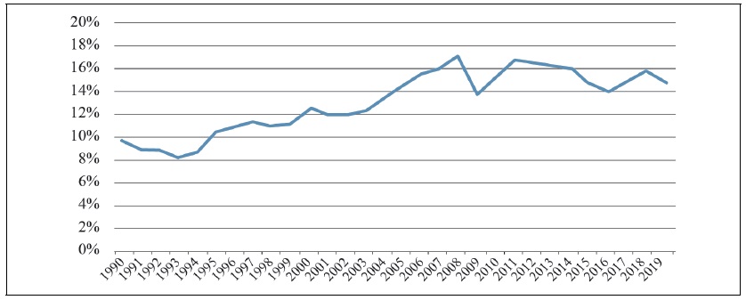
Figure 2 compares the world trend with the GII of East Asian economies. For the world, the GII index has different values as compared to Figure 1 due to different data sources (with ICIO tables measuring trade from a national account perspective). However, the trend over time is the same. All East Asian economies have a decreasing import intensity since the financial crisis. But Figure 2 highlights that China follows a different trend with the decrease starting before other countries and being more severe. Due to its economic size, China plays an important role in the decrease of the world average.
China was initially a country involved in processing trade and assembly activities in GVCs (Xing, 2016). Such specialization involved high levels of imports of intermediate inputs, explaining a high GII in 2005. The economic size of countries has an impact on their use of imported inputs. Small economies cannot manufacture domestically the full range of intermediate goods and services needed. They have to rely more on imports, as illustrated with Hong Kong, China and Chinese Taipei in Figure 2. Large economies, in contrast, can find locally a variety of inputs and have lower values for the GII, as illustrated with Japan. In 2005, China had a very high GII compared to its size and started to converge towards a level more in line with those observed in large economies. Concretely, this means that instead of importing intermediate products, China has increasingly relied on its domestic producers of inputs. These producers have caught up with their foreign competitors and some upgrading took place, allowing China to produce with a higher domestic content (Duan et al., 2018) as high quality inputs can now be found in the domestic economy. Wen (2018) indicates that the Chinese domestic value added in exports has not increased and was actually still decreasing at the beginning of the 2010s. But the share of domestic value added coming from upstream sectors has significantly increased.
However, Figure 2 points to a decrease in the GII for other East Asian economies, including Korea and Japan that were not on the same development path as China. The world decline is generally discussed in the context of concerns about globalization, rising trade tensions and a new wave of technological progress (the digital transformation and advanced robotics) that may not lead to further fragmentation of production. Therefore, the difficulty is to disentangle the causes of the decline observed in China.
2. Changes in Final Demand Versus the Structure of GVCs
Figure 3 relies on the decomposition of equation (2) in section II to distinguish changes in GVC structure from changes in final demand in the evolution of global imports between 2011 and 2016. During this period, changes in world imports were mostly related to a reduction in the fragmentation of production and less related to composition effects in final demand. This result is a bit different from Timmer et al. (2016) who found that in 2011-2014, changes in fragmentation and in final demand contributed roughly equally to the decline in GII. It comes from the fact that we use more recent data (including revisions for previous years) and a dataset with more countries that can better capture structural changes. Data in Timmer et al. (2016) were already suggesting that the reduction in the fragmentation of production was prevalent in 2013-2014 and this is even more the case after 2014 in our dataset.
Changes in final demand include shifts in the demand for products, for example from manufactured goods (with long value chains) to services (that are produced in shorter value chains) or shifts in the shares of countries in world demand (with different levels of involvement in GVCs). Such changes in the structure of final demand explain a small portion of the change in the overall import intensity at the world level between 2011 and 2016. But in East Asia, the situation is different with China having not only an important decrease in its imports related to the structure of GVCs but also an almost equal decrease due to changes in final demand. Korea and to a lower extent Hong Kong and Chinese Taipei are also economies where the shift in final demand is significant, although still lower than the change due to the fragmentation of production. Only Japan follows a different trend with a smaller decrease in import intensity related to GVC structure and a slight increase in imports related to changes in final demand. It is in the most developed countries that the fragmentation of production is the main driver of the GII decline, as observed also in the United States and the European Union (explaining the result for the world on Figure 3).
For countries with still high growth rates, it is not surprising to see that the change in final demand accounts for a significant part of the change in GII. For example, consumers within China are likely to change the type of products they import as their income increases. Moreover, a higher share of China in world final demand should also contribute to changes in imports related to what China consumes and what other countries export to China. Nevertheless, such change and the fact that it contributes negatively to the growth of imports can also suggest that rising trade tensions have affected trade in final products as much as trade in intermediate inputs.
At the industry level, Figure 4 provides further insights into composition versus structural effects in the reorganization of GVCs in China, Japan and Korea. Korea is the country where the import intensities have declined the most, particularly in industries where the fragmentation of production was high, such as the other transport equipment industry (a sector that includes shipbuilding) and the motor vehicles industry. 5 This trend may reflect some upgrading and technological shifts. For example, shipbuilders in Korea have engaged in active backward linkages and functional upgrading strategies to increase the domestic content of ships (Brun and Frederick, 2017). In the motor vehicles industry, vertical integration and the increasing importance of electronic components in cars can also explain shorter value chains in Korea (Choi and Choi, 2016). Such trends are not a cause of concern if driven by productivity gains and technological change. However, economic inefficiencies can arise if changes are driven by increased trade costs that make domestic producers artificially competitive.
In Japan, the fragmentation of production has not decreased in most industries, including in the ICT and electronics sectors and the motor vehicles industry where GVCs are the most prevalent. It is rather in traditional industries subject to new competition from emerging economies, such as basic and fabricated metals that GVCs have become shorter.
In China, there is more heterogeneity across industries. An important decline in the GII index is observed in the textiles and apparel industry, as well as chemicals, basic metals and ICT & electronics. These industries are the ones were domestic upgrading occurred and where new Chinese brands have started to replace the manufacturing of products for foreign companies, together with the development of competitive domestic input suppliers. There is evidence of functional upgrading when looking at the type of jobs embodied in the products of Chinese GVCs that are increasingly related to R&D, logistics, sales, marketing, back-office services and less related to fabrication activities (Timmer et al., 2019; de Vries et al., 2019).
5)The evolution of the coke and petroleum industry might be influenced by price effects (variations in the price of oil as an input for this industry). ICIO tables are in current prices. Import intensities are ratios and are not affected by the overall evolution of prices but are still sensitive to variations in relative prices across products.
IV. EVOLUTION OF TRADE COSTS ALONG THE VALUE CHAIN
From the above analysis, we have seen that the fragmentation of production has decreased in East Asia, with the exception of Japan. Now the question is whether this is the result of technology-led changes in business models and productivity-enhancing adjustments to value chains or the consequence of policies that would have increased the cost of offshoring. In particular, any impact of a change in policies should be reflected in trade costs. We can expect technological progress to continue to decrease trade costs (through reduced transport and communication costs) or to be neutral when leading to new business models changing patterns of trade based on other costs than those associated with international trade. Barriers to trade related to geography, language or culture are also not expected to change when considering a short period of time. Raising trade costs in 2011-2016 would be the sign that new barriers to trade and investment or changes in the regulatory environment have reduced opportunities for benefiting from offshoring and international sourcing.
1. Bilateral Trade Costs
Figure 5 plots the average bilateral trade costs in East Asia together with a world average. The country with the lowest trade costs is China. This does not mean that it is the country with the most liberal trade policies as trade costs encompass all types of costs, including transport costs that are related to geography. Moreover, it should be recalled that the trade cost index we use is based on the geometric average of trade costs in both directions. The relatively low value for China can also indicate that other countries are open to trade with China. The index is also a tariff equivalent, meaning that a value of 1.05 for China in 2016 is the equivalent of a 105% tariff when adding all types of barriers to trade (i.e. tariffs, non-tariff measures, transport costs, costs related to geography and culture, etc.). This approach leads to high levels of trade restrictions and a different hierarchy across countries as compared to a simple comparison of tariffs, for example.6
This being said, both Korea and China have trade costs that are below the world average while Japan and Chinese Taipei have slightly higher trade costs. Hong Kong is the economy with the highest trade costs, due in particular to its specialization in services that generally face higher trade costs (Miroudot et al., 2013).
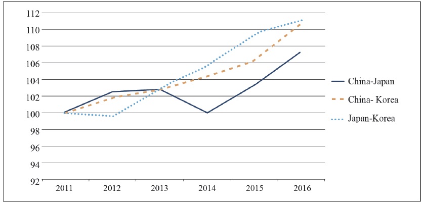
To understand whether trade costs have been impacted by a change in the policy environment since 2011, Figure 6 looks at an index of the evolution of bilateral trade costs with the value of 100 in 2011. The use of such an index makes the results less sensitive to the parameter of the model and offers a better comparison over time for countries starting from different levels of trade costs.
Figure 6 suggests some volatility in the evolution of average bilateral trade costs in East Asia. It is interesting to see an increase in China and Korea, and possibly Japan in the most recent period, as it could be associated to rising trade tensions. Regionalism was among the main drivers of the rise of GVCs in the 2000s in East Asia (Pomfret, 2010). Economic integration has continued in the 2010s, particularly with ASEAN economies, but some authors describe a slowdown in regionalism and possibly more tensions with China (Yeo, 2020). Until the recent signature of the Regional Comprehensive Economic Partnership (RCEP), there was also no trade agreement covering bilateral trade between China, Japan and Korea, despite the ‘CJK’ negotiations. Combined with the lack of multilateral trade liberalization since the failure of the Doha Round and an increase in the use of protectionist measures and state interventions since the financial crisis (Evenett, 2019), rising trade costs are not surprising and may have affected East Asia through partner countries, if not through trade restrictions put in place in the region.
Figure 7 provides a closer look at the China-US bilateral relationship. In addition, to the index previously calculated as a geometric average of bilateral trade costs in both directions, the simple unidirectional index (total trade costs) is also provided based on equation (8). We use this second approach to answer the question of whether trade costs on exports from the US to China or exports from China to the US have changed (and having in mind that our data are until 2016, i.e. before the recent ‘trade war’).
Figure 7 indicates that with the exception of the financial crisis, bilateral trade costs between China and the US have decreased, even after 2011 and the start of the first trade tensions. Only the last year in the dataset suggests a change (in 2016). There are higher trade costs for exports from the US to China than exports from China to the US. And the decrease in trade costs is on China’s side when looking at the unidirectional total trade costs measure. But when adding the general equilibrium effects (i.e. the impact of multilateral resistance terms), there is no upward trend in 2016, suggesting that, if confirmed, this upward trend would be directly related to a change in the trade environment between China and the US and not to changes in relative prices and trade flows with other countries.
If before 2016, there was no significant change in China-US bilateral trade costs, the increase in average trade costs observed in Figure 6 comes from other bilateral relationships. Figure 8 suggests that trade costs have actually increased within East Asia. The level of bilateral trade costs between China, Japan and Korea is generally lower than the average (due to geographic proximity) but there is a steady increase in these trade costs after 2011. While no significant change in trade policy can explain this increase, it should be noted that the measure we use can be influenced by tensions between countries and perceptions of businesses. As per equation (7), the index increases when intra-national trade becomes relatively higher than international trade. Moreover, distortions affecting trade are increasingly outside the traditional scope of trade policy and related to government support, such as subsidies (OECD, 2019).
2. Cumulative Trade Costs
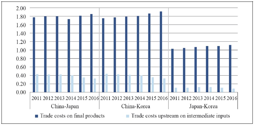
The cumulative trade costs, calculated with equation (9), can give more insights into whether upstream trade costs are responsible for rising trade costs within East Asia. Figure 9 shows the bilateral trade costs on final products and the cumulative impact of trade costs on intermediate inputs used to produce these final products for China, Japan and Korea. Trade costs are higher for final products by construction because the full value of products is subject to these costs. Trade costs upstream come from imported inputs that account for a small share of output and shares of imported inputs become smaller and smaller when moving up the value chain (through the multiplication by the A matrix as described in Section II). Cumulative trade costs tend to be higher in bilateral relationships involving China and it is true both for trade costs on final products and for inputs used to manufacture them.
But what Figure 9 suggests is that the increase in bilateral trade costs that was observed in Figure 8 is driven by trade costs on final products. They have increased in the three bilateral relationships. Along the value chain, there is on the contrary a decrease in cumulative trade costs for inputs used to manufacture final products exchanged between China, Japan and Korea (although less pronounced for Japan-Korea). Therefore, while the decrease of global imports of final products could be explained by increased trade costs, the evidence suggests that in terms of the structure of GVCs, other drivers may be responsible for the lower levels of fragmentation of production in East Asia.
As discussed in Section III, technological shifts and upgrading can explain a productivity-enhancing decrease in the fragmentation of production. For example, producers of final products can first rely on foreign suppliers for specialized inputs while focusing on assembly activities. Once they accumulate skills and know-how and have the financial capacity to invest in new technologies and capital, they can internalize the production of inputs, which is one aspect of functional upgrading. This process certainly plays a role in China and to a lesser extent in Korea. But technological change can also lead to shorter value chains in the context of the digitalization of economies and servitization, when business models require producing closer to consumers and rely more on intangible assets than physical value chains. It could explain that countries that are no longer upgrading their actitivities in GVCs also experience a decrease in the fragmentation of production (such as Japan).
With a methodology similar to the calculation of trade costs along the value chain, productivity can also be analyzed from a GVC perspective (Dietzenbacher and Los, 2012), accounting for productivity not only in the final industry but also in industries producing inputs. Results for East Asia (with data up to 2014) highlight that GVC productivity has steadily increased and that the productivity increase comes from intermediate input industries (including services) and not just from final production (Miroudot, 2019). These data are consistent with a productivity-enhancing decrease in the fragmentation of production.
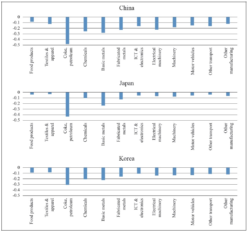
At the industry level, the decrease in trade costs on inputs in GVCs is confirmed for the main manufacturing industries in China, Japan and Korea (Figure 10). The decrease is the highest in the coke and petroleum industry, followed by basic metals. It means that inputs used in these industries (including services inputs) are coming from countries with decreasing bilateral trade costs (which have themselves sourced inputs from countries with decreasing bilateral trade costs). Food products, textiles & apparel, ICT & electronics and other transport equipment are the industries where the reduction in cumulative trade costs was the lowest. Across all industries, China is the country that has generally benefited from lower trade costs upstream. This evidence does not point to a particular problem with trade costs and rising protectionism on trade in inputs needed for the manufacturing of final products in East Asia.
This result is not inconsistent with increased protectionism through government support or subsidies, as such policies would aim at lowering costs for domestic producers and would increase trade costs on the final products either directly through measures put in place by partner countries in retaliation or indirectly by making exports of partner countries less competitive. We observed the raising trade costs on final products within East Asia on Figure 8.
6)Note also that this figure depends on the choice of sigma, the elasticity of substitution across products. While the literature suggests lower values for sigma, it exponentially increases the level of bilateral trade costs in the formula we use.
V. WHAT HAS COVID-19 CHANGED?
COVID-19 has caused a series of disruptions in GVCs related to health measures put in place by governments to contain the spread of the virus. Some of these measures have been temporary (such as the lockdowns in some countries that have closed down production in some industries), while others are still implemented (such as restrictions on travel and quarantines). Only data for 2020 could allow a precise analysis of these disruptions on GVCs. However, even if COVID-19 is a crisis that has no ending date at this stage, the discussion on the future of GVCs is more about how companies will reorganize their value chains after the crisis and whether this reorganization will be influenced by new approaches towards risks in the supply chain.
Several authors have suggested that some companies will reconsider complex international value chains, as well as just-in-time production strategies (Javorcik, 2020; Shih, 2020). GVCs might become shorter and more domestic. However, there is very little empirical evidence supporting such a change. In the past, companies that have faced major natural disasters have not tried to reduce the internationalization of production. For example, after the 2011 T?hoku earthquake and tsunami in Japan, Zhu et al. (2016) and Matous and Todo (2017) find some evidence of supplier diversification but leading to more offshoring. The international business literature also indicates that firms manage risks through capabilities such as agility, flexibility and supply chain visibility and not by reorganizing their value chains to avoid risks (Miroudot, 2020). These capabilities allow firms to anticipate disruptions and to quickly react to mitigate their impact.
The consequences of COVID-19 might be different but on economic grounds, there is no change in costs that would justify shorter value chains or a reshoring of production. On the contrary, model simulations suggest the opposite. Reshoring would lead both to lower levels of GDP and a higher volatility of output (Bonadio et al., 2020; OECD, 2020).
As it was observed for bilateral trade costs during the Great Financial Crisis (for example in Figure 5), a short-term increase in trade costs will be recorded and corresponding to the higher freight rates and disruptions in transport networks experienced during COVID-19. Depending on how long the virus will be actively circulating, this increase might be higher and more persistent (particularly for trade in services that depends on movement of people). But these higher trade costs should disappear after the crisis.
If there is a long-term impact of COVID-19, it is more likely to happen through a change in policy-making that would accentuate protectionism. For example, instead of companies naturally reshoring production to reduce their exposure to risk, reshoring could be triggered by policies giving economic incentives to firms to produce locally (e.g. subsidies) and discouraging imports of inputs or final goods produced abroad (e.g. tariffs). We have previously mentioned the trend towards the use of new types of trade barriers more oriented towards subsidies and government support. However, as highlighted in Section IV, these barriers may have explained rising trade costs on final products but were not found to have significantly changed cumulative trade costs along the value chain, including in industries where such support is more common.
A difference after COVID-19 could be increased pressure and more incentives for the localization of the production of inputs (in line with the argument that it would reduce risks in the value chain). This trend would lead to different results as those observed in Section IV with possibly rising cumulated trade costs in GVCs. It would accentuate the reduction in the fragmentation of production but with a different driver than in 2011-2016.
However, it is not clear that governments will be successful in implementing policies leading to reshoring and the localization of production at a large scale. Such policies involve distortions that are costly and impede on the competitiveness of firms. Such policies will be resisted by the private sector and gains from multinational production and offshoring will remain, giving a competitive edge to companies still producing in GVCs.
Finally, COVID-19 could also accelerate the digital transformation with teleworking, e-commerce and other digital technologies becoming more popular. And it is not clear at this stage whether it will benefit the fragmentation of production or not. On the one hand, digital technologies can increase the connectivity between countries and favor offshoring and international trade networks (Obashi and Kimura, 2020). But on the other hand, they can also lead to a new division of labor between developed and developing countries involving less offshoring (Baldwin, 2016).
VI. CONCLUDING REMARKS
This paper has reviewed evidence on the reorganization of GVCs in East Asia using the OECD inter-country input-output tables and looking at the global import intensity of production and trade costs along the value chain. The main trends identified are the following.
There is a decrease in the fragmentation of production in East Asia since 2011, which is more pronounced than in the rest of the world. To produce the same output, East Asian economies rely less on imported intermediate inputs and value chains have become shorter. The explanation is both within East Asian economies and in economies supplying inputs to East Asian producers. Within East Asia, China has changed the composition of its final demand and is increasingly relying on domestic input suppliers, a shift that started before 2011. But other economies have also reduced their global import intensity. While we observe increasing trade costs within East Asia, this trend is fully driven by trade in final goods. There is no evidence that trade costs along the value chain have increased for firms producing in East Asia in 2011-2016.
This result implies that other trends and other types of costs (not related to trade) are behind the reduction in the fragmentation of production. If companies rely less on offshoring and imported inputs in the context of decreasing trade costs in the value chain, it suggests a process driven more by efficiency-enhancing strategies or the reduction of domestic costs than constraints related to the international trade and investment environment. This is in line with changes in GVCs related to the digital transformation and new business models of firms producing closer to consumers.
However, due to the important time lag in the release of input-output statistics, we could only provide this evidence up to 2016 and without covering the most recent trade tensions related to the US-China ‘trade war’. As COVID-19 is likely to intensify trade and investment uncertainties, trade costs –that have increased during the crisis due to trade disruptions- could remain at a high level on a more long-term basis in the post-COVID world. To avoid this, policies aimed at reducing uncertainties and preserving the gains from multilateral and regional trade and investment liberalization will be important in the recovery phase. If cumulative trade costs have not increased in GVCs in East Asia, there was evidence of rising trade costs on final products that could prevent trade from fully contributing to future growth.
Finally, an econometric panel analysis of the change in the fragmentation of production that would include as independent variables the change in bilateral trade costs but also additional variables reflecting technological change and other determinants of the length of value chains could be an avenue for future research.
Tables & Figures
Figure 1.
Global import intensity of production (1990-2019)
Source: OECD, COMTRADE and IMF.
Figure 2.
Global import intensity of production (2005-2016): world and East Asian economies
Source: Author’s calculations based on OECD ICIO tables, 2018 edition.
Figure 3.
Decomposition of the change in global import intensity: GVC structure and final demand, 2011/2016, log points
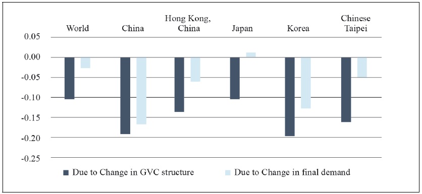
Source: Author’s calculations based on OECD ICIO tables, 2018 edition.
Figure 4.
Global import intensity for manufacturing industries: 2016 versus 2011
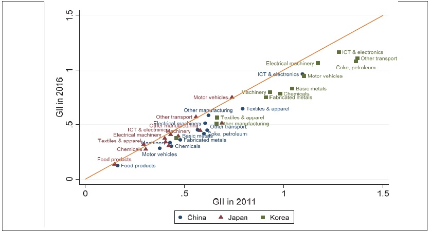
Source: Author’s calculations based on OECD ICIO tables, 2018 edition.
Figure 5.
Average bilateral trade costs, 2005-2016, tariff equivalent
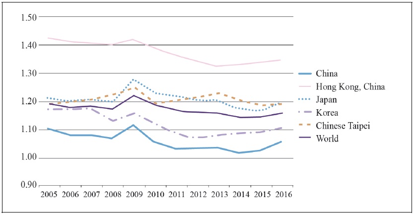
Source: Author’s calculations based on OECD ICIO tables, 2018 edition. Trade costs are aggregated across countries and partner countries through production and expenditure shares.
Figure 6.
Change in average bilateral trade costs since 2011, 2011=100
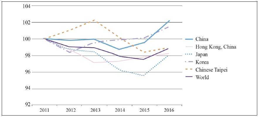
Source: Author’s calculations based on OECD ICIO tables, 2018 edition. Trade costs are aggregated across countries and partner countries through production and expenditure shares.
Figure 7.
A closer look at China-US trade costs, 2005-2016
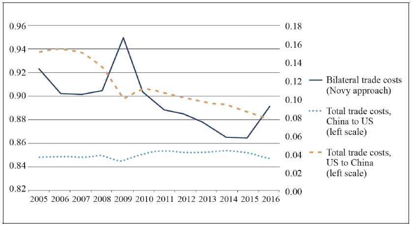
Source: Author’s calculations based on OECD ICIO tables, 2018 edition.
Figure 8.
Bilateral trade costs between China, Japan and Korea, 2011=100
Source: Author’s calculations based on OECD ICIO tables, 2018 edition.
Figure 9.
Cumulative trade costs between China, Japan and Korea, 2011-2016, tariff equivalents
Source: Author’s calculations based on OECD ICIO tables, 2018 edition.
Figure 10.
Cumulative trade costs on inputs for selected manufacturing industries: 2016 versus 2011, % points
Source: Author’s calculations based on OECD ICIO tables, 2018 edition.
References
- Agnosteva, D. E., Anderson, J. E. and Y. V. Yotov. 2014. Intra-National Trade Costs: Measurement and Aggregation. NBER working paper, no. 19872.
-
Anderson, J. E. and E. van Wincoop. 2003. “Gravity with Gravitas: A Solution to the Border Puzzle,”
American Economic Review , vol. 93, no. 1, pp. 170-192.
-
Anderson, J. E., Larch, M. and Y. V. Yotov. 2018. “GEPPML: General Equilibrium Analysis with PPML,”
World Economy , vol. 41, no. 10, pp. 2750-2782.
-
Anderson, J. E. and Y. V. Yotov. 2010. “The Changing Incidence of Geography,”
American Economic Review , vol. 100, no. 5, pp. 2157-2186.
-
Baldwin, R. 2006. “Globalisation: The Great Unbundling(s).” In
Globalisation challenges for Europe . Part I. Helsinki: Secretariat of the Economic Council. pp. 11-54. -
Baldwin, R. 2016.
The Great Convergence: Information Technology and the New Globalization . Cambridge, MA: Harvard University Press. -
Baldwin, R. and R. Forslid. 2014. “The Development and Future of Factory Asia.” In Ferrarini, B. and D. Hummels. (eds.)
Asia and Global Production Networks. Implications for Trade, Incomes and Economic Vulnerability . Cheltenham: ADB and Edward Elgar. pp. 338-368. -
Baldwin, R. and T. Okubo. 2019. “GVC Journeys: Industrialisation and Deindustrialisation in the Age of the Second Unbundling,”
Journal of the Japanese and International Economies , vol. 52, pp. 53-67.
- Bonadio, B., Huo, Z., Levchenko, A. A. and N. Pandalai-Nayar. 2020. Global Supply Chains in the Pandemic. NBER Working Paper, no. 27224.
- Brun, L. and S. Frederick. 2017. “Chapter 4. Korea and the Shipbuilding Global Value Chain.” In Korea in Global Value Chains: Pathways for Industrial Transformation. Duke Global Value Chains Center and Korea Institute for Industrial Economics & Trade.
-
Caliendo, L. and F. Parro. 2015. “Estimates of the Trade and Welfare Effects of NAFTA,”
Review of Economic Studies , vol. 82, no. 1, pp. 1-44. -
Choi, B.-I. 2020. “Global Value Chains in East Asia under ‘New Normal’: Ideology-Technology-Institution Nexus,”
East Asian Economic Review , vol. 24, no. 1, pp. 3-30. -
Choi, S.-H. and J.-I. Choi. 2016. “GVC Case Analysis of the Motor Vehicles Industry: Focusing on Hyundai Motor,”
Journal of Digital Convergence , vol. 14, no. 12, pp. 73-84. (in Korean)
-
de Vries, G., Chen, Q., Hasan, R. and Z. Li. 2019. “Do Asian Countries Upgrade in Global Value Chains? A Novel Approach and Empirical Evidence,”
Asian Economic Journal , vol. 33, no. 1, pp. 13-37. -
Dietzenbacher, E., and B. Los. 2012. “Quantification of the Contributions of Productivity Growth and Globalization to World Consumption Growth Rates (1995-2008).” Paper presented at the 32nd General Conference of the International Association for Research in Income and Wealth. Boston. August.5-11, 2012. <
http://www.iariw.org/papers/2012/LosPaper.pdf > (accessed March 21, 2020) -
Duan, Y., Dietzenbacher, E., Jiang, X., Chen, X. and C. Yang. 2018. “Why Has China's Vertical Specialization Declined?”
Economic Systems Research , vol. 30, no. 2, pp. 178-200. -
Eaton, J. and S. Kortum. 2002. “Technology, Geography, and Trade,”
Econometrica , vol. 70, no. 5, pp. 1741-1779. -
Evenett, S. J. 2019. “Protectionism, State Discrimination, and International Business since the Onset of the Global Financial Crisis,”
Journal of International Business Policy , vol. 2, no. 1, pp. 9-36. -
Head, K. and J. Ries. 2001. “Increasing Returns versus National Product Differentiation as an Explanation for the Pattern of U.S.-Canada Trade,”
American Economic Review , vol. 91, no. 4, pp. 858-876.
-
Head, K. and T. Mayer. 2014. “Gravity Equations: Workhorse, Toolkit, and Cookbook.” In Gopinath, G., Helpman, E. and K. Rogoff. (eds.)
Handbook of International Economics . vol. 4. Amsterdam: Elsevier. pp. 131-195. -
Javorcik, B. 2020. “Global Supply Chains Will Not Be the Same in the Post-COVID-19 World.” In Baldwin, R. and S. J. Evenett. (eds.)
COVID-19 and Trade Policy: Why Turning Inward Won’t Work . London: CEPR Press. pp. 111-116. -
Johnson, R. C. 2018. “Measuring Global Value Chains,”
Annual Review of Economics , vol. 10, pp. 207-236.
-
Leontief, W. W. 1936. “Quantitative Input and Output Relations in the Economic System of the United States,”
Review of Economics and Statistics , vol. 18, no. 3, pp. 105-125.
-
Matous, P. and Y. Todo. 2017. “Analyzing the Coevolution of Interorganizational Networks and Organizational Performance: Automakers’ Production Networks in Japan,”
Applied Network Science , vol. 2, article no. 5, pp. 1-24. <https://doi.org/10.1007/s41109-017-0024-5> ; (accessed March 21, 2020)
- Miroudot, S. 2019. Services and Manufacturing in Global Value Chains: Is the Distinction Obsolete? ADBI Working Paper Series, no. 927.
-
Miroudot, S. 2020. “Reshaping the Policy Debate on the Implications of COVID-19 for Global Supply Chains,”
Journal of International Business Policy , vol. 3, no. 4, pp. 430-442. -
Miroudot, S. and H. Nordström. 2020. “Made in the World? Global Value Chains in the Midst of Rising Protectionism,”
Review of Industrial Organization , vol. 57, no. 2, pp. 195-222. -
Miroudot, S. and M. Ye. 2020. “Decomposing Value Added in Gross Exports,”
Economic Systems Research . <https://doi.org/10.1080/09535314.2020.1730308 > (accessed May 30, 2020) - Miroudot, S., Rouzet, D. and F. Spinelli. 2013. Trade Policy Implications of Global Value Chains: Case Studies. OECD Trade Policy Paper, no. 161.
-
Miroudot, S., Sauvage, J. and B. Shepherd. 2013. “Measuring the Cost of International Trade in Services,”
World Trade Review , vol. 12, no. 4, pp. 719-735.
-
Novy, D. 2013. “Gravity Redux: Measuring International Trade Costs with Panel Data,”
Economic Inquiry , vol. 51, no. 1, pp. 101-121.
-
Obashi, A. and F. Kimura. 2018. “Are Production Networks Passé in East Asia? Not Yet,”
Asian Economic Papers , vol. 17, no. 3, pp. 86-107.
- Obashi, A. and F. Kimura. 2020. New Developments in International Production Networks: Impact of Digital Technologies. ERIA Discussion Paper Series, no. 332.
-
Organisation for Economic Co-operation and Development (OECD). 2013.
Interconnected Economies. Benefiting from Global Value Chains . Paris: OECD Publishing. - Organisation for Economic Co-operation and Development (OECD). 2019. Measuring Distortions in International Markets: The Semiconductor Value Chain. OECD Trade Policy Papers, no. 234.
-
Organisation for Economic Co-operation and Development (OECD). 2020.
Shocks, Risks and Global Value Chains: Insights from the OECD METRO model . Paris: OECD Publishing. -
Pomfret, R. 2010.
Regionalism in East Asia: Why Has It Flourished Since 2000 and How Far Will It Go? Hackensack: World Scientific Publishing. -
Shih, W. 2020. “Is It Time to Rethink Globalized Supply Chains?”
MIT Sloan Management Review , vol. 61, no. 4, pp. 16-18. -
Taglioni, D. and D. Winkler. 2016.
Making Global Value Chains Work for Development . Washington, DC: The World Bank. -
Timmer, M. P., Erumban, A. A., Los, B., Stehrer, R. and G. J. de Vries. 2014. “Slicing Up Global Value Chains,”
Journal of Economic Perspectives , vol. 28, no. 2, pp. 99-118. - Timmer, M. P., Los, B., Stehrer, R. and G. J. de Vries. 2016. An Anatomy of the Global Trade Slowdown based on the WIOD 2016 Release. GGDC Research Memorandum, GD-162.
-
Timmer, M. P., Miroudot, S. and G. J. de Vries. 2019. “Functional Specialization in Trade,”
Journal of Economic Geography , vol. 19, no. 1, pp. 1-30.
-
Wen, D. 2018. “Domestic Value Added in China’s Exports to the World and its Partners,”
Chinese Economy , vol. 51, no. 1, pp. 45-68. -
World Bank. 2019.
World Development Report 2020. Global Value Chains: Trading for Development . Washington, DC: The World Bank. -
Xing, Y. 2016. “Global Value Chains and China’s Exports to High-Income Countries,”
International Economic Journal , vol. 30, no. 2, pp. 191-203.
-
Yeo, A. 2020. “China’s Rising Assertiveness and the Decline in the East Asian Regionalism Narrative,”
International Relations of the Asia-Pacific , vol. 20, no. 3, pp. 445-475.
- Zhu, L., Ito, K. and E. Tomiura. 2016. Global Sourcing in the Wake of Disaster: Evidence from the Great East Japan Earthquake. RIETI Discussion Paper Series, no. 16-E-089.