

- EAER>
- Journal Archive>
- Contents>
- articleView
Contents
Citation
| No | Title |
|---|---|
| 1 | Parasal Aktarım Mekanizması Kanallarından Faiz ve Kredi Kanalının VAR Yöntemiyle İncelenmesi: Türkiye Örneği / 2022 / European Journal of Science and Technology |
Article View
East Asian Economic Review Vol. 25, No. 1, 2021. pp. 73-97.
DOI https://dx.doi.org/10.11644/KIEP.EAER.2021.25.1.391
Number of citation : 1View
75
Download
65
Evolution of China’s Economy and Monetary Policy: An Empirical Evaluation Using a TVP-VAR Model
|
|
Department of Economics, Chonnam National University |
|---|

Abstract
China has experienced many structural changes in the process of economic development over the past three decades. Using a time-varying parameter VAR model with stochastic volatility and mixture innovations, this study investigates whether such structural changes in, especially tools and operational aims of monetary policy, affect the monetary transmission mechanism. We find that impulse responses of output growth and inflation to monetary shocks have substantially increased and then reversed to decrease around 2005-2006. This time variation is mainly caused by changes in the monetary transmission mechanism, i.e., the manner in which main macroeconomic variables respond to policy shocks, rather than by changes in volatilities of exogenous shocks. The result implies that aggressive monetary policy to facilitate economic growth in the developing economies may be legitimized, unless it causes inflation seriously.
JEL Classification: E52, E30, C11
Keywords
Monetary Policy, Evolution of Transmission Mechanism, Stochastic Volatility, Time-Varying Impulse Responses
I. Introduction
China has achieved unprecedentedly high economic growth over the past three decades and is now the second largest economy in the world. It is well known that improvement of institutional arrangements has played important roles in the process of the economic growth in China: the instructional improvement was crucial sometimes because high economic growth has been facilitated by transformation of the Chinese economy from a socialistic system to more market-oriented system. A long list of such institutional improvements may be presented. However, development and improvement of a monetary policy framework is of special interest in the current study. Two features can be identified in the evolution of the monetary policy framework. First, the monetary policy regime evolved from direct to more indirect control (see, e.g., Xie, 2004 and Sun, 2013). For example, the People’s Bank of China (PBC) used mainly the credit quota to support allocation of resources in accordance with the central government’s plan. Since 2000, however, the PBC has transferred to a regime of more market-oriented policy tools, such as targeting to the growth rate of monetary aggregate. Second, the priority of monetary policy has changed from supporting economic growth to stabilizing the economy (see e.g. Zheng et al., 2012; Girardin et al., 2014 and Chen and Huo, 2009). Such changes in institutional arrangements and policy priority may cause changes in the transmission mechanism of monetary policy, i.e., the manner in which main macroeconomic variables respond to policy shocks. This study tries to examine this speculation by tracing out the evolution of the monetary policy transmission mechanism in China over the last three decades.
If the PBC has changed its operating framework of monetary policy substantially over time, its monetary policy reaction function may not be well described with any time-invariant equation. We use a time-varying parameter vector autoregressive (TVP-VAR) model with stochastic volatility. The TVP-VAR models are relatively new, but they are now increasingly used in empirical macroeconomic literature. The salient analysis using the VAR model with time-varying coefficients was developed by Cogley and Sargent (2001) and further improved by other scholars (notably, Sims and Zha, 2006; Cogley and Sargent, 2005 and Primiceri, 2005). We use the mixture innovation model, an extended model nesting the class of TVP-VAR models with stochastic volatility, proposed by Koop et al. (2009). There are advantages in using the mixture innovation model, and some of them may not be trivial in the current context. The mixture innovation model is more flexible than the typical TVP-VAR model, because it can encompass various modes of structural breaks, including two extremes: time-varying parameter (TVP) models and regime-switch models. The regime change in the TVP models, by set up, occurs every time period, and the magnitude of the change is restricted typically to be small. Conversely, the regime change in regime-switch models occurs infrequently, but its magnitude is usually not restricted. The evolution of the monetary policy framework of China has sometimes been gradual but has been drastic at other times, as China transfers from a centrally planned economy to a more market-oriented economy. As seen later, for example, the major reform of the institutional arrangements is concentrated on specific years, around 1998. On the other hand, monetary policy priority has changed gradually from growth supporting to stabilizing the economy in the 2000s. This mixed nature of regime changes can be captured more properly by the mixture innovation TVP model rather than by conventional TVP models.
In spite of the increasing importance of China in the world economy, not enough research effort on China’s monetary policy has been attempted, because of the lack of reliable macroeconomic data covering a long-enough period, especially a GDP series. Chang et al. (2015) apply some interpolation methods to official data and construct a main macroeconomic time series of monthly and quarterly frequencies. This study takes advantage of their datasets and provides some important findings about the effects of China’s monetary policy undocumented by previous studies.
We find that there was a turning point in the impulse responses to a monetary shock around 2005-2006: the responses of output and inflation to a positive monetary shock increased and then decreased around this period. Such change in impulse response function has been made gradually sometimes and relatively drastically at other times. This is consistent with the argument of the mixed nature of regime changes. Changes of the operating framework of monetary policy might alter private agent decisions and, as a consequence, the dynamics of the macroeconomic variables and transmission mechanism of monetary shocks, as argued by rational expectation economists like Sargent (1984). We also present evidence suggesting that monetary policy has been more inflation-stabilizing in recent periods than in early periods. This is consistent with the previous findings and the current argument that monetary policy evolves from the growth-supporting regime to the inflation-stabilizing regime.
Given evidence that regime changes occur in the impulse responses of major macroeconomic variables to monetary shocks over time, we examine the main causes of such regime changes. Changes in impulse responses can be caused by either changes in the transition mechanism of monetary shocks, i.e., the way in which macroeconomic variables respond to shocks, as represented by VAR coefficients, or changes in the way in which the exogenous shocks are generated, i.e., variance-covariance of the shocks in the current context. The mixture innovation model allows both time-varying VAR coefficients and time-varying variance-covariance of exogenous shocks in a flexible and robust manner. We can, thus, examine effectively the primary channels for the changes in impulse response functions. We estimate two supplementary VAR models: the VAR model with time-varying VAR coefficients, but constant variance-covariance; and the VAR model with stochastic volatility, but constant VAR coefficients. The result implies that the time variation in the impulse responses of output growth and inflation is mainly attributable to stochastic VAR coefficients rather than the stochastic volatility of exogenous shocks. Many developed countries, notably, the US and the UK, experienced so-called ‘great moderation’ over the last few decades before the breakout of the international financial crisis in 2008: better performance of major macroeconomic variables with lower volatility (see, e.g., Stock and Watson, 2002 for the US and Benati, 2008 for the UK). However, most of the literature casts doubts on the role that monetary policy had in shaping the observed changes in the US.: this difference in performance reflects mainly the heteroscedasticity of the exogenous shocks, which were much more volatile in the 1970s and 1980s (see Blanchard and Simon, 2001; Stock and Watson, 2002; Primiceri, 2005; Sims and Zha, 2006 and Canova and Gambetti, 2009). However, China is different: it is a transition economy that has been experiencing many structural changes in the economy, including institutional arrangements. This aspect of a transition economy may cause changes in the transmission mechanism of monetary shocks.
Our result indicates that impulse response of GDP growth to monetary shocks exhibits hump-shaped time variation parallel to actual GDP growth. This confirms again that the underlying cause of the time variation of the impulse response is mainly changes in transmission mechanism of monetary shocks. The parallel movement also implies that aggressive monetary policy to foster economic growth or to address economic hardship may be legitimized, unless it causes inflation seriously.
The remainder of this paper is organized as follows. Section II briefly reviews how the Chinese economy and monetary policy evolved over the last three decades. Section III provides some preliminary results estimated from the conventional linear VAR models. Section IV explains the core aspects of the mixture innovation model. Section V reports the results of impulse response analysis for the evolution of the transmission mechanism of monetary policy. Our conclusions are presented in section VI.
II. The Evolution of China’s Economy and Monetary Policy Framework
As is well known, China was a centralized planned economy before the 1980s. Economic resources were mainly allocated by the central government rather than by market operation. However, China’s economy staggered under the centralized system. In the 1980s, China started to open the door to the world and launched a series of economic reform programs to boost economic growth. One part of the economic reform was to improve institutional arrangements to be more like those of market economies. In the current context, special attention should go to the monetary policy framework. The PBC was the only bank before the 1980s, and its main function was supporting allocating resources in accordance with the central government’s plan. In 1984, the regular commercial banking activities were separated from the PBC and passed to four newly established state-owned commercial banks. The PBC was designated exclusively as a central bank. The objectives of monetary policy of the PBC were defined in the People’s Bank of China Act promulgated in 1995 as “to maintain the stability of the value of the currency and thereby promote economic growth”. The growth target is set each year by the central government to guarantee enough job creation to absorb the consistent labor surplus, mainly freed from the agricultural sector. The PBC has thus attached great importance to economic growth corresponding to the growth target. Another reform of the framework of monetary policy was implemented in 1996: the PBC introduced the growth rates of monetary aggregates (M1 and M2) as nominal anchors and adopted them, together with the credit quotas, as its intermediate targets. A series of important reforms of the operating system of monetary policy were implemented in 1998: bank-specific credit quotas were formally abolished in January and, instead, the PBC started to set the target for total bank lending and used it as one of its intermediate targets as well; the PBC resumed the open market operations. There is thus a broad consensus in the literature that the year 1998 was a turning point of the PBC’s monetary policy regime from direct to more indirect control (see, e.g., Xie, 2004), although to some degree, direct monetary control methods still exist.
There is much literature arguing that there were regime shifts in the policy priority in the 2000s. Zheng et al. (2012) provide evidence that the policy response to inflation was larger during 1998-2002 than in previous periods, implying that the PBC paid increased attention to inflation. Girardin et al. (2014) examine China’s monetary policy reaction to inflation for the period of 2002-2013. They conclude that the PBC appears to have built up a monetary policy framework similar to implicit flexible inflation targeting, and that the PBC’s behavior post-2002 resembles that of the post-1979 anti-inflation policy of the G3 central banks, albeit with a high output weight typical of emerging economies. Girardin et al. (2017) examine the monetary policy of the PBC by Taylor rule and conclude that regime change in the policy rule happened in 2002: the policy rule before 2002 is characterized by a relatively expansionary approach to price stability; by contrast, policy in recent periods features a relatively contractionary approach. Chen and Huo (2009) also find structural changes in the Chinese monetary policy rule around 1998 and 2002-2003.
The episode about the evolution of the economy and monetary policy may be reflected in the data. Figure 1 plots the evolution of the main macroeconomic series since 1979. It appears that three regimes may be identified in association with changes in economic conditions and monetary policy stances from 1990 to the recent period. China’s economy took off in the 1980s, and the real GDP growth rate was maintained at around 10% except for large drops during the political turmoil in 1989-1990. However, inflation increased dramatically in the second half of the 1980s, from 2.7% in 1984 up to 17.2% in 1988. Consequently, China’s economy experienced high economic growth and high inflation in the beginning of the 1990s: the inflation rate increased from 9.7% in Jan. 1993 up to 24.4% in Oct. 1994. The first regime covers roughly the period of 1993-1997. Drastic monetary contractions against such a rocket of inflation were implemented: the M2 growth rate was reduced from about 35% in 1993 to about 15% in 1997. The inflation rate was reduced, possibly with this drastic monetary contraction: the inflation rate dropped below 10% in 1995 and further to 5% in 1997. In short, the first regime features strong monetary contractions to suppress inflation.
The benchmarking deposit rate decreased from 10.98% to 7.47% in 1996 and 5.67% in 1997 to mitigate the adverse effects of contractionary M2 growth on GDP growth. Nonetheless, China’s economy experienced a steady slowdown in economic growth during the period of the first regime. The central government needed to boost economic growth to guarantee enough job creation to absorb the consistent labor surplus, mainly freed from the agricultural sector. The second regime thus started with a reversal of monetary policy stance, from contractionary to boosting economic growth. M2 growth was maintained at around 12~13% around the beginning of 2000, but it increased up to 19.5% in 2003. Afterward, M2 growth repeated ups-and-downs with an upward trend. The expansionary policy stance was also reflected in low interest rates: the benchmarking deposit rate was maintained between 1.98% and 2.25% during the period from June 1999 to July 2006.
Economic growth dropped to about 7% at the end of 2008 and up to 6.7% in 2009 as the international financial crisis hit China’s economy. The year 2009 is recorded as the most drastic monetary expansion period except for some initial years. M2 growth rocketed up to 26% at the end of 2009. However, the monetary expansions ended shortly and the final regime is characterized by a downward trend of M2 growth and GDP growth. Inflation touched up to 6.3% in 2011. Since then it has decreased and stabilized at around 1~2% recently. At the same time, the GDP growth rate decreased after reaching 10.2% and has fluctuated at around 6.5% recently. Thus the final regime appears to be consistent with the previous argument, that the priority of monetary policy moved from a growth supporting to more stabilizing regime. Girardin et al. (2017) construct a monetary policy index and show that the policy style moves from inflation-accommodating to anti-inflation policy from 2002 onwards. Zheng et al. (2012) also find similar policy changes, concluding that the PBC paid increased attention to inflation.
In sum, it is a rational speculation that changes in operational efficiency of monetary policy, changes in policy priority, and possibly, other structural changes facilitating the process of the liberalization and transformation of the Chinese economy may cause changes in the transmission mechanism of monetary policy shock since the 1990s.
III. Some Preliminaries
One may cast doubt on the quality of the official macroeconomic data of China, especially the GDP series. However, Chen et al. (2016) argue that official GDP figures remain a useful and valid measure of Chinese economic activities. They use annual macroeconomic data and construct a monthly and quarterly series of GDP and other macroeconomic data by applying some interpolation methods. We believe that their monthly dataset is the most reliable one among the existing datasets and thus we need not attempt any formal tests on the quality. Nonetheless, we want to confirm that the interpolated data is useful in the current context, on the one hand, and that the VAR model used for the current empirical study represents China’s macroeconomy well reasonably, on the other hand. Moreover, since China is still a communist country, at least officially, one may raise a question: Does such a monetary policy typical for Western economies exist in China? One indirect way to examine the quality of data is to see if the estimation result of the VAR models is reasonable compared with theories and previous studies.
We estimate impulse responses from a conventional linear VAR model as reported in Figure 2. The model includes the same lag order and the same four endogenous variables as the TVP-VAR model: real output, CPI, real effective exchange rate (REER), and M2. We transform monthly data into year-on-year growth by taking log-difference. As expected, GDP growth increases in response to a positive shock to M2 growth. The CPI inflation also increases and thus, use of M2 representing the stance of monetary policy does not cause the so-called “price puzzle”—as noted by Sims (1992)—where a rise of monetary growth reduces the inflation rate. 1 The real effective exchange rate increases in the first month, but decreases afterward, implying that exports become cheaper in response to monetary expansions. This is also consistent with expectation.
It is known that the PBC has multiple instruments of monetary policy. Thus it may be plausible to include other tools of monetary policy into the model, especially interest rates. The VAR model in Figure 3 includes two additional variables: seven-day repo rate and one-year benchmarking deposit rate. The impulse responses of GDP, inflation, and REER to a positive shock to M2 growth estimated from the extended VAR model are pretty similar with those from the four-variable model. The impulse responses of shocks to interest rates are of interest, too. The 7-day repo rate decreases in response to a monetary expansion as expected, even though the confidence band includes zero response. On the other hand, the one-year benchmarking deposit rate increases. This may reflect that the PBC pursues sometimes two (possibly conflicting) aims using different policy tools: it reduces M2 growth to stabilize inflation, whereas it lowers the interest rate to boost economic growth.2 TVP-VAR models of many variables are not feasible in general, because of the computational burden, and the present study is thus parsimonious in selecting endogenous variables of the VAR model. However, the estimation results from Figure 2 and Figure 3 imply that the parsimonious model represents China’s macroeconomy reasonably well.
1)Using short-term interest rate such as 7-day repo rate of benchmarking lending rate, 1year deposit rate exhibits the price puzzle even though the results are not reported here.
2)We estimate impulse responses to a positive shock to the interest rate even though we do not report the results to save space. Our result confirms that the interest rate is not a proper instrument of monetary policy stance, being consistent with the argument of the previous studies such as
IV. The Model
Koop et al. (2009) propose a TVP-VAR model with stochastic volatility and mixture innovation nesting the class of TVP-VAR models. The TVP-VAR model is estimated by the same MCMC (Monte Carlo and Markov Chain) algorithm proposed by Primiceri (2005). Koop et al. (2009) add additional steps for the mixture innovation aspect of the model. For the purpose of brevity, we do not replicate every step of the estimation procedure and instead summarize the core aspects of the model. For technical details of the estimation procedure, readers can refer to Primiceri (2005) and Koop et al. (2009).
Consider the following state-space representation form of the VAR model:

where 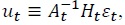 where
where
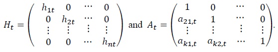
Stacking the autoregressive terms, the model is simplified as:

where 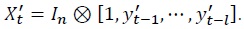 The state representation is characterized as the following state equations:


The parameters in the mixture innovation model, defined as equations (3) through (5), can either remain constant (
Previous TVP models can be nested by this mixture innovation extension of the TVP-VAR with stochastic volatility. The model used by Primiceri (2005) can be considered a special case with restrictions
For a linear VAR, impulse responses can be directly taken from the vector moving average (VMA) representation implied by the VAR. However, with a TVP-VAR, the implied VMA representation continues to change over time. Suppose that the implied VMA is given by:
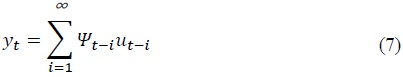
Impulse responses at time

where
V. Empirical Results
1. Variables and Data
Bayesian estimation of TVP-VAR models requires exorbitant calculation, and hence large systems are usually not feasible. We try to balance between the two conflicting objectives: minimizing the number of variables included in the model and representing China’s economy reasonably by the model. The resultant VAR model includes four endogenous variables: real GDP growth, CPI-inflation, change in real effective exchange rate (REER), and M2 growth rate.3 The data are monthly figures, and all growth variables are year-on-year changes in log to guarantee stationarity, as reported in Table 1. Real effective exchange rate4 is included to reflect the fact that foreign trade plays important roles in the process of economic development in China. The ordering is assumed to be recursive: monetary policy reacts contemporaneously to output growth and inflation shocks, but it has no contemporaneous effect on output growth and inflation. This structural interpretation is intuitively appealing, at least for the monthly frequency data, and it is a standard assumption used by many others. The ordering has also practical benefits—MCMC draws of
M2 growth acts as a proxy variable representing the stance of monetary policy. The PBC uses multiple instruments of monetary policy. However, there are several reasons that quantity-based instruments are better measures of monetary policy stance than are price-based instruments. First of all, several institutional arrangements do not develop enough that the normal interest-rate channel fails in the monetary transmission mechanism. Since bond markets in China are not fully developed, long-term interest rates for investment are largely insulated from changes in short-term interest rates. Lending and deposit rates in the banking system have not been fully liberalized to react the risk to bank loans (Chen et al., 2016). Thus, much literature argues that the interest rate is not a proper proxy for the monetary stance (e.g., Fan et al., 2011). The previous section above also indicates that using the interest rate as a proxy for monetary policy does not yield reasonable figures for impulse response functions.
We use dataset constructed by Higgins et al. (2016), which was last updated in 2018. They use official data and construct the monthly dataset by applying interpolation as proposed by Chow and Lin (1971). Our dataset covers the periods from 1993:1 to 2018:4.
2. Evolution of the Effects of Monetary Policy: Impulse Response Analysis
Given our speculation that the evolution of institutional arrangements and monetary policy framework may have affected the time variation of the effect of monetary policy, we focus on impulse responses to a positive monetary shock. The responses are the effect of a shock of size one to the structural errors and they can be directly compared over time. Figure 4 indicates that a positive shock to M2 growth has hump-shaped effects on GDP growth and inflation, which is similar to the cases of the linear VAR models. The figure also shows that REER appreciates in a short initial period and then depreciates in response to a positive shock to M2 growth. This is also similar with the result estimated from the linear VAR models. The effects of monetary shocks, especially on GDP growth and inflation, vary substantially over time. Figure 5 paints a picture of the time variation of the impulse responses to expansionary monetary shocks. The response of GDP growth does not exhibit substantial time variation in the 1990s. However, it increases during the first half of the 2000s and touches a maximum in 2005 or 2006. Afterward, the response of GDP growth decreases until recent years. The response of inflation fluctuates a lot over time. Nonetheless, the similar pattern of time variation is also observed, even though it is less vivid than is the response of output: the response of inflation increases until around 2006 or 2007 and then decreases. This pattern of time variation of impulse responses of output and inflation appears to be consistent with the previous studies, such as Zheng et al. (2012) and Girardin et al. (2014): they provide evidence that regime changes in monetary policy stance happened around 2003 from growth boosting to stabilization. Time variation of impulse responses of M2 growth is also consistent with the argument of more stabilization in the recent period: monetary policy shocks are less persistent in the 2010s than in the previous period as implied in the last picture of Figure 5. This stabilization trend reminds of the great moderation of developed countries in 1980s and 1990s. However, the case of China is different, in the sense that the stabilization is accompanied by a downward trend of economic growth, whereas the developed countries experienced better economic growth.
Finally, it is worth noting that an expansionary monetary shock has had more profound impacts on REER recently. This appears at first to be in contrast to the current finding that its effects on output and inflation have been weaker recently. In order to be integrated into the world economy, however, the Chinese government has targeted improvements in the international financial market represented by the Renminbi (RMB) exchange rate market. Especially, the government has strengthened the marketizations of RMB exchange rate and capital accounts and hence the RMB exchange rate has recently been more volatile in recent period.5 The profound effects on REER may reflect this improvement of the international financial market as the monetary shock becomes more pass-through to the exchange rate under the environment of more marketization of the RMB exchange rate and capital account.
3. Causes for the Changes in the Effect of Monetary Policy
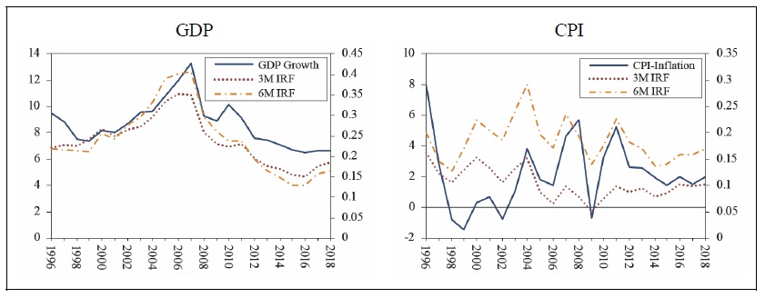
Given the finding that the effect of monetary shocks represented by the impulse responses has changed substantially over time, what are the underlying causes for such time variation? Does the time variation reflect a transmission mechanism of monetary shocks possibly caused by structural changes of China’s economy, such as changes of the framework of monetary policy? Or is it just coincidence, reflecting changes in the volatility of exogenous shocks? Following Koop et al. (2009), we refer to the manner in which the exogenous shocks affect the variables of interest as the transmission mechanism. For example, the great moderation of the US economy may be due to good monetary policy. In this case, the great moderation is an example of a change in the transmission mechanism of the policy shocks. Conversely, if the great moderation is mainly due to the variance of less volatile exogenous shocks, it is an example of the good luck story. In Figure 6, we compare actual time series of GDP growth and of inflation with impulse responses to a monetary shock as estimated from the previous subsection. The figure indicates that the impulse response of GDP growth follows remarkably closely the time path of actual GDP growth. CPI inflation also reveals some parallel movement with actual inflation series, even though it appears to be much less clear than in the case of GDP growth. The parallel movement between impulse responses and actual series can be interpreted at least as evidence against a good luck story: it is hard to believe that the hump-shaped time variation of the impulse responses is a result of coincidental time variation of variance of exogenous shocks. Furthermore, China is a transition economy and the hump-shaped time variation of actual GDP growth may be a result reflecting features specific to the transition economy, such as changes in institutional arrangements and monetary policy frameworks. Taking this speculation given, the parallel movement between, especially, the impulse responses and the actual GDP growth can be interpreted as an example of a story of changes in transmission mechanism of monetary shocks. This argument can be supported further by Figure 7. The figure indicates that the volatility of exogenous shocks to GDP growth decrease substantially during the 2010s. The reduction of volatility of exogenous shocks is also observed in M2 growth and inflation equations, even though it is much less vivid. This implies that recent stabilization of the economy may be attributable at least in part to the reduction of volatility of exogenous shocks of the VAR equations. However, the time variation of the variance of exogenous shocks is unlikely to be a main cause for the hump-shaped time variation of impulse responses of GDP and inflation to monetary shocks.
The argument about relative importance of changes in transmission mechanism of monetary shocks and variance of exogenous shocks can be examined more rigorously by controlling the time variation of the VAR coefficients or variance-covariance matrix. We estimate impulse responses from the two supplementary models in Figure 8: the VAR model with stochastic VAR coefficients, but constant variance-covariance, that is,
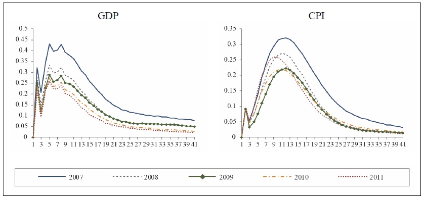
Finally, changes in transmission mechanism of monetary shocks in times of economic crises or financial turmoil may be of interest, too. For example, Azariadis and Smith (1998) argue that the economy can switch back and forth cyclically between a Walrasian regime in expansions and a credit-rationing regime in contractions. Ravn and Sola (2004) also argue that monetary policy might have real effects in crisis time through credit and liquidity channels, whereas monetary shocks during booms are close to neutral in effect. Extensive empirical research has been devoted to examining the nonlinearity of monetary policy in association with economic turmoil or business fluctuations (e.g., Weise, 1999; Garcia and Schaller, 2002; Lo and Piger, 2005 and Balke, 2000). The previous research typically finds that monetary policy has greater effects in times of business recessions or financial turmoil than in normal times. China experienced unprecedentedly large drops in GDP growth in 2009 and Chen et al. (2016) also find similar evidence for China. However, we cannot find evidence consistent with the previous studies. Figure 10 focuses on impulse responses in the period around 2009 of economic shortfall, but provides no picture in favor of the evidence that the effects of monetary policy are stronger in the periods around 2009. One possible explanation for the different result from the previous findings can be found from the fact that the drastic monetary expansions to address the economic slowdown in the crisis period last only shortly: M2 growth touched 26.0% in November in 2009, but it reduced to the pre-crisis level in June in 2010 and decreased steadily afterward. In fact, ignoring the period around the 2009-crisis, M2 growth rate has a long-run downward trend since 2005. This long-trend may dominate short-term changes in monetary policy and the possible regime change in the effect of monetary policy around 2009 may not be identified.
3)We extended the lag order up to 5, but the result does not change substantially. Including more lags leads to inaccurate estimation as too many parameters should be estimated. The order of the VAR variables is recursive. The result is sensitive when the policy variable M2 is not ordered last. However, different order of non-policy variables does not affect the result substantially. Thus, our result is robust enough to lag orders and order of VAR variables.
4)The real effective exchange rate is calculated as weighted averages of bilateral exchange rates adjusted by relative consumer prices (Bank for International Settlements, Real Broad Effective Exchange Rate for China).
5)Major events of the reform are: In 1994, a single managed floating exchange rate system was established to eliminate the dual exchange rate system; China joined the WTO in 2001; In 2007, a quote-driven market making system was established and the daily volatility of the RMB exchange rate against the US dollar in the interbank market was expanded from plus or minus 0.3% to plus or minus 0.5%. The floating range of the interbank spot exchange rate was expanded to 1% in 2012 and it was expanded further from 1% to 2% in 2014. Refer to
VI. Conclusion
In the presence of structural changes in the interrelationship between major macroeconomic variables, evaluating monetary policy often poses challenges to researchers. This may be much true for a transition economy like China as it is likely to experience important structural changes over the past three decades in the process of transition from a centrally planned system to a market-oriented system. Particularly, the framework of monetary policy has transformed from the regime of direct control to more indirect and market-oriented regime, and operational priority of monetary policy has moved from a growth-supporting regime to an inflation-stabilizing regime. We speculate that such structural changes and operational regime changes of monetary policy may affect the transmission mechanism of monetary shocks. We find evidence in favor of this speculation.
In our study, the effect of monetary policy, represented by impulse responses, changes over time: the responses of output growth and inflation to positive monetary shocks increase and then decrease over time. It is shown that the time variation of impulse responses is more attributable to changes in the monetary transmission mechanism, the manner in which variables of interest respond to exogenous shocks, rather than the time variation of the variance of exogenous shocks, even though both are important. We also find some evidence supporting the view that the operational aim of monetary policy has moved from a growth-supporting regime to an inflation-stabilizing regime. The parallel movement between the impulse responses and the actual time series implies an important policy insight. Aggressive monetary policy to support economic growth in the developing economies may be legitimized, unless it causes seriously inflation.
Tables & Figures
Figure 1.
Real GDP Growth, Inflation and Money Growth
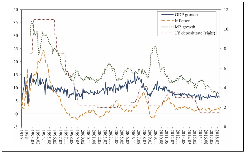
Note: GDP growth and CPI-inflation before 1993 constructed from annual data, otherwise all series except the deposit rate are year-on-year growth constructed from monthly figures.
Figure 2.
Impulse Responses to a Monetary Shock: Estimated from the Conventional VAR
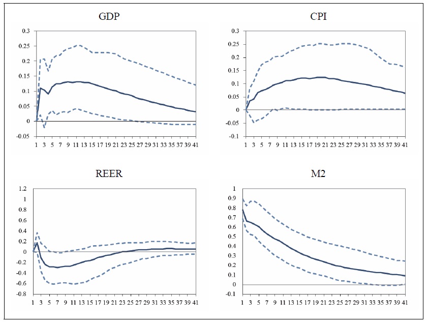
Figure 3.
Impulse Responses to a Monetary Shock: Estimated from the 6-Variable VAR
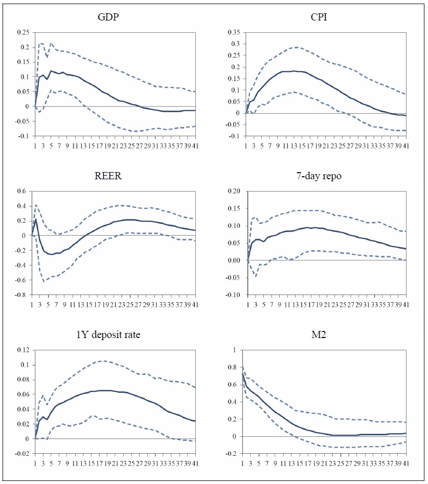
Table 1.
Unit Root Tests
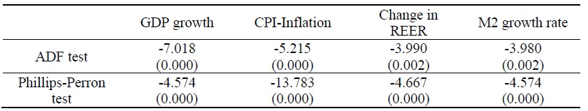
Note: p-values are reported in parenthesis.
Figure 4.
Impulse Responses to a Monetary Shock: Estimated from the TVP-VAR with Mixture Innovation
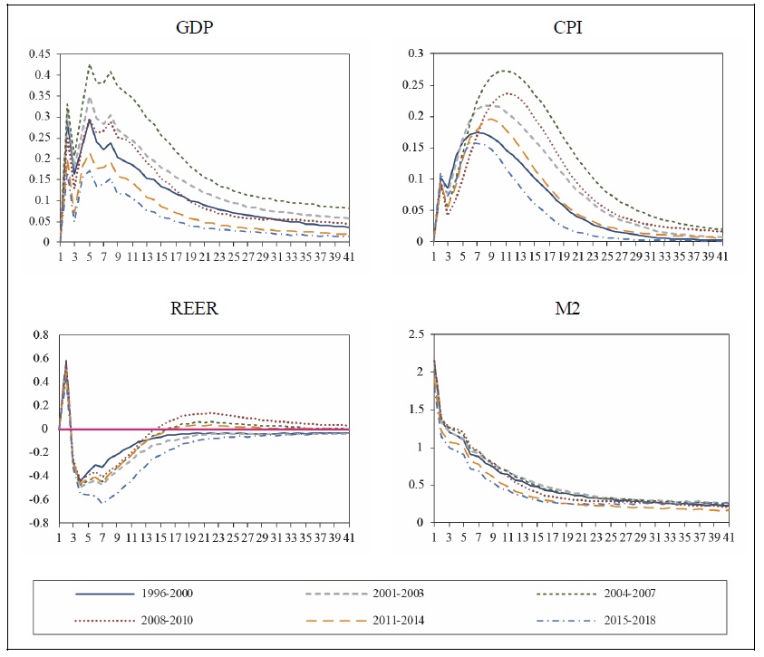
Figure 5.
Long-Run Trend of Impulse Responses to a Monetary Shock: One-Year Averages
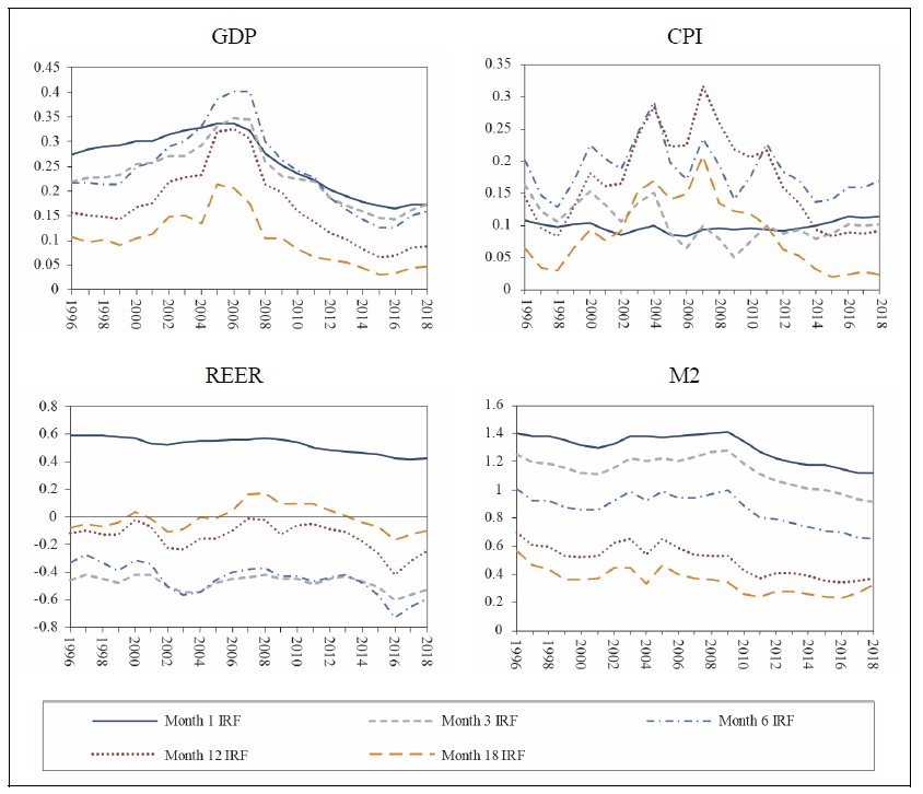
Figure 6.
Impulse Responses and Actual Time Series
Note: Impulse responses functions are right scale. GDP growth and CPI-inflation are calculated as twelvemonth average of year-on-year growth of monthly figures.
Figure 7.
Standard Deviation of Residuals Estimated from the TVP-VAR with Mixture Innovation Model
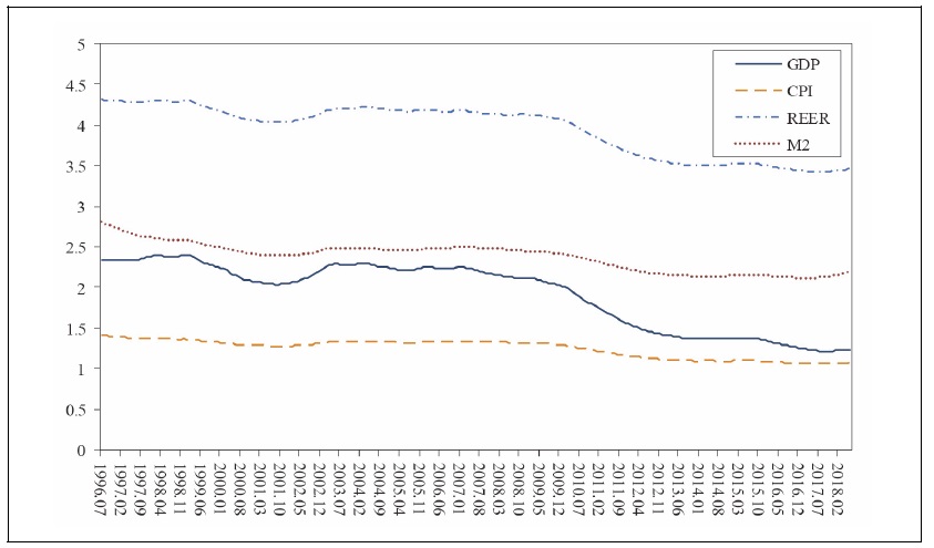
Figure 8.
Impulse Responses to a Monetary Shock: CS-VAR Models Vs Hetero-VAR Models
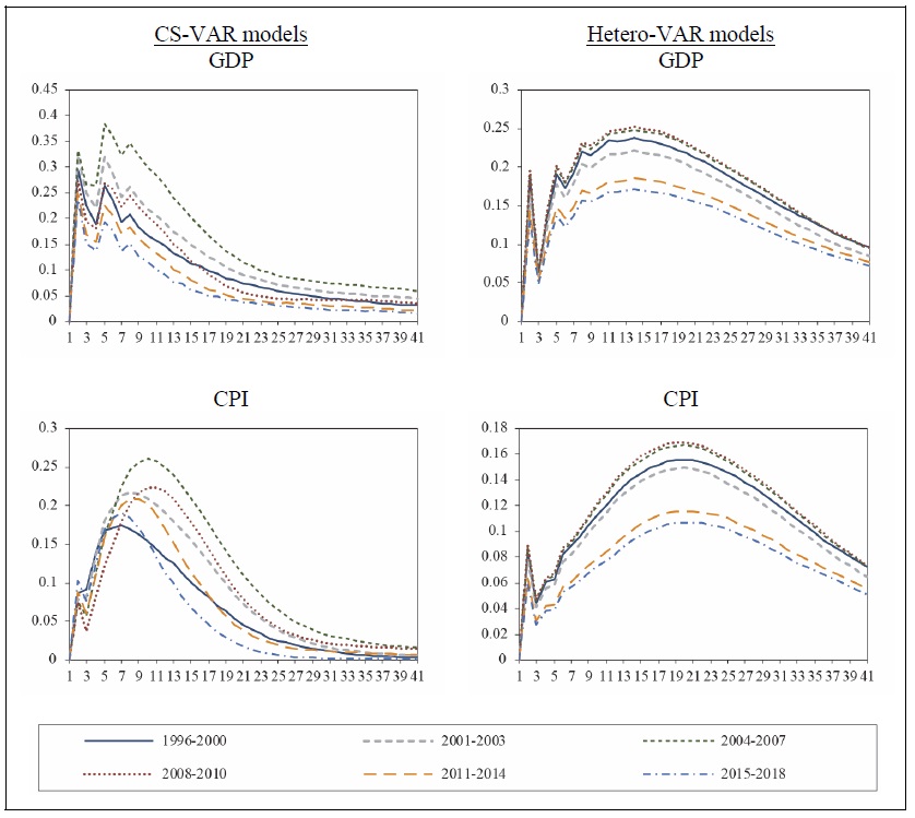
Figure 9.
Impulse Responses to a Monetary Shock Rstimated from Alternative Models
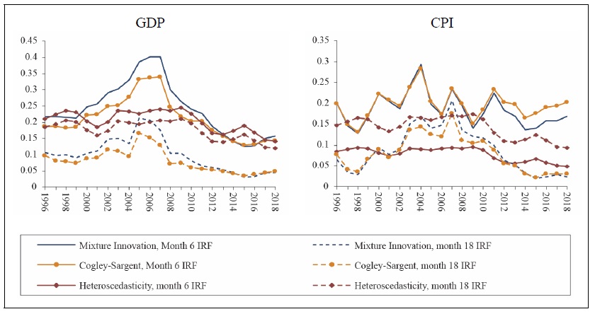
Figure 10.
Impulse Responses to a Monetary Shock around 2009
References
-
Azariadis, C. and B. Smith. 1998. “Financial Intermediation and Regime Switching in Business Cycles,”
American Economic Review , vol. 88, no. 3, pp. 516-536. -
Balke, N. S. 2000. “Credit and Economic Activity: Credit Regimes and Nonlinear Propagation of Shocks,”
Review of Economics and Statistics , vol. 82, no. 2, pp. 344-349.
-
Benati, L. 2008. “The Great Moderation in the United Kingdom,”
Journal of Money, Credit and Banking , vol. 40, no. 1, pp. 121-147.
-
Blanchard, O. and J. Simon. 2001. “The Long and Large Decline in U.S. Output Volatility,”
Brookings Papers on Economic Activity , vol. 2001, no. 1, pp. 135-164.
-
Canova, F. and L. Gambetti. 2009. “Structural Changes in the US Economy: Is There a Role for Monetary Policy?”
Journal of Economic Dynamics & Control , vol. 33, no. 2, pp. 477-490.
-
Chang, C., Chen, K., Waggoner, D. and T. Zha. 2015. “Trends and Cycles in China’s Macroeconomy.” In Eichenbaum, M. and J. A. Parker. (eds.)
NBER Macroeconomics Annual 2015 , vol. 30. Chicago: University of Chicago Press. pp. 1-84. - Chen, K., Higgins, P., Waggoner, D. and T. Zha. 2016. Impacts of Monetary Stimulus on Credit Allocation and Macroeconomy: Evidence from China. NBER Working Papers, no. 22650.
-
Chen, K., Ren, J. and T. Zha. 2018. “The Nexus of Monetary Policy and Shadow Banking in China,”
American Economic Review , vol. 108, no. 12, pp. 3891-3936.
-
Chen, Y. and Z. Huo. 2009. “A Conjecture of Chinese Monetary Policy Rule: Evidence from Survey Data, Markov Regime Switching, and Drifting Coefficients,”
Annals of Economics and Finance , vol. 10, no. 1, pp. 111-153. -
Chow, G. C. and A. Lin. 1971. “Best Linear Unbiased Interpolation, Distribution, and Extrapolation of Time Series by Related Series,”
Review of Economics and Statistics , vol. 53, no.4, pp. 372-375.
-
Cogley, T. and T. J. Sargent. 2001. “Evolving Post-World War II U.S. Inflation Dynamics.” In Bernanke, B. S. and K. Rogoff. (eds.)
NBER Macroeconmics Annual 2001 , vol. 16. Cambridge, MA: MIT Press. pp. 331-373. -
Cogley, T. and T. J. Sargent. 2005. “Drifts and Volatilities: Monetary Policies and Outcomes in the post WWII U.S,”
Review of Economic Dynamics , vol. 8, no. 2, pp. 262-302.
-
Fan, L., Yu, Y. and C. Zhang. 2011. “An Empirical Evaluation of China’s Monetary Policies,”
Journal of Macroeconomics , vol. 33, no. 2, pp. 358-371.
-
Garcia, R. and H. Schaller. 2002. “Are the Effects of Monetary Policy Asymmetric?”
Economic Inquiry . vol. 40, no. 1, pp. 102-119.
- Girardin, E., Lunven, S. and G. Ma. 2014. Inflation and China’s Monetary Policy Reaction Function: 2002–2013. BIS Papers, no. 77.
- Girardin, E., Lunven, S. and G. Ma. 2017. China’s Evolving Monetary Policy Rule: From Inflation-Accommodating to Anti-Inflation Policy. BIS Working Papers, no. 641.
-
Higgins, P., Zha, T. and W. Zhong. 2016. “Forecasting China’s Economic Growth and Inflation,”
China Economic Review , vol. 41, pp. 46-61.
-
Koop, G., Leon-Gonzalez, R. and R. W. Strachan. 2009. “On the Evolution of the Monetary Transmission Mechanism,”
Journal of Economic Dynamics and Control , vol. 33, no. 4, pp. 997-1017.
-
Koop, G., Pesaran, M. H. and S. M. Potter. 1996. “Impulse Response Analysis in Nonlinear Multivariate Models,”
Journal of Econometrics , vol. 74, no. 1, pp. 119-147.
-
Lo, M. C. and J. Piger. 2005. “Is the Response of Output to Monetary Policy Asymmetric? Evidence from a Regime-Switching Coefficients Model,”
Journal of Money, Credit and Banking , vol. 37, no. 5, pp. 865-886.
-
Primiceri, G. E. 2005. “Time Varying Structural Vector Autoregressions and Monetary Policy,”
Review of Economic Studies , vol. 72, no. 3, pp. 821-852.
-
Ravn, M. O. and M. Sola. 2004. “Asymmetric Effects of Monetary Policy in the United States,”
Federal Reserve Bank of St. Louis Review , vol. 86, no. 5, pp. 41-60. -
Ren, Y., Yang, Y. and X. Zhong. 2015. “Effect of Currency Exchange Rate on Economic Growth-Research Based on RMB Exchange Rate of VAR Model.” In
Proceedings-2nd International Conference on Education, Management and Information Technology, October 10-11, 2015 . Atlantis Press. pp. 467-472. -
Sargent, T. 1984. “Autoregressions, Expectations, and Advice,”
American Economic Review , vol. 74, no. 2, pp. 408-415. -
Sims, C. A. 1992. “Interpreting the Macroeconomic Time Series Facts: The Effects of Monetary Policy,”
European Economic Review , vol. 36, no. 5, pp. 975-1011.
-
Sims, C. A. and T. Zha. 2006. “Were There Regime Switches in U.S. Monetary Policy?”
American Economic Review , vol. 96, no. 1, pp. 54-81.
- Stock, J. H. and M. W. Watson. 2002. Has the Business Cycles Changed and Why? NBER Working Papers, no. 9127.
-
Sun, R. 2013. “Does Monetary Policy Matter in China? A narrative Approach,”
China Economic Review , vol. 26, pp. 56-74.
-
Weise, C. L. 1999. “The Asymmetric Effect of Monetary Policy: A Nonlinear Vector Autoregression Approach,”
Journal of Money, Credit, and Banking , vol. 31, no. 1, pp. 85-108.
- Xie, P. 2004. China’s Monetary Policy: 1998-2002. King Center on Global Development Working Papers, no. 217. Stanford University.
-
Zheng, T., Wang, X. and H. Guo. 2012. “Estimating Forward-Looking Rules for China’s Monetary Policy: A Regime-Switching Perspective,”
China Economic Review , vol. 23, no. 1, pp. 47-59.