

- EAER>
- Journal Archive>
- Contents>
- articleView
Contents
Citation
| No | Title |
|---|
Article View
East Asian Economic Review Vol. 20, No. 2, 2016. pp. 169-190.
DOI https://dx.doi.org/10.11644/KIEP.EAER.2016.20.2.308
Number of citation : 0View
952
Download
556
Are Korean Industry-Sorted Portfolios Mean Reverting?
|
|
Department of Economics, Chonbuk National University |
|---|

Abstract
This paper tests the weak-form efficient market hypothesis for Korean industry-sorted portfolios. Based on a panel variance ratio approach, we find significant mean reversion of stock returns over long horizons in the pre Asian currency crisis period but little evidence in the post-crisis period. Our empirical findings are consistent with the fact that Korea accelerated its integration with international financial market by implementing extensive capital liberalization since the crisis.
JEL classification: G14, G11, G10
Keywords
Mean Reverting, Panel Variance Ratio Tests, Efficient Market Hypothesis, Industry-sorted Stock Price Indexes
I. INTRODUCTION
This paper tests the weak-form efficient market hypothesis for Korean stock markets. The weak-form efficient market hypothesis implies that stock returns are not predictable using past returns. A well-known alternative to this hypothesis is the mean reversion hypothesis stating that stock prices tend to return a trend path in the long run. In empirical finance, many studies test the efficient market hypothesis, using various empirical methods and data sets, and report mixed evidence on the predictability of stock returns, in particular for mean reversion in long horizons.
For example, Fama and French (1988, p. 538) report that “25-45 percent of the variation of 3-to 5-year stock returns is predictable from past returns,” using monthly data of US stock prices in the 1926-85 period. Porteba and Summers (1988) find similar results of mean reversion over long horizons.1 In contrast, Richardson and Stock (1989) show that the univariate variance ratio tests employed in previous studies are not consistent when the return horizon is large relative to sample size and generate negative biases. Once these biases are corrected, they find little evidence of mean reversion even in long horizons in contrast to Fama and French (1988) and Porteba and Summers (1988).2 As summarized in Campbell et al. (1997), one difficulty in using long horizon returns (multi-year returns) for testing efficient market hypothesis and for detecting mean reversion is the very small sample size: standard econometric tests generally lack of power to reject the null hypothesis that stock prices follow a random walk process against the alternative of mean reversion.
In this paper, we use panels of KOSPI industry group stock portfolio indexes for the period of 1988-2016 and of KOSDAQ industry group stock portfolio indexes for the period of 2001-2016. The use of panels mitigates the small sample size problems because they contain additional information in cross-industry variations. The idea of using a panel data set in testing the predictability of stock prices is from Balvers et al. (2000) who examine mean reversion using a panel of stock price indexes for 18 countries with well-developed capital markets (16 OECD countries plus Hong Kong and Singapore) in the period of 1969-1996 and find strong evidence of mean reversion. Gropp (2004) also follow Balvers et al. (2000) and employ a panel of 16 US industry-sorted portfolios for the period of 1926-1998 and find evidence of mean reversion in industry stock price indexes. Following Fama and French (1988) and Gropp (2004), we use industry group stock portfolio indexes, rather than using size-sorted portfolios (classified by market capitalization) which have been widely used in previous studies. The reason for this selection is related to one key difference between industry-sorted portfolios and size-sorted portfolios: stocks with abnormal high or low returns tend to move across portfolios from one year to next in the latter. Therefore, if abnormal performance of stocks is caused by temporary shocks, subsequent price reversals would be missed and thus detection of mean reversion would be underestimated. On the other hand, stocks in general do not move across portfolios in the former.
To test the weak-form efficient market hypothesis using the panel data sets, we use panel variance ratio tests recently developed by Moon and Velasco (2014). Variance ratio tests have been widely used to detect mean reversion in long horizon returns in various asset markets such as stock and currency markets.3 However, the use of the tests has been limited only for univariate time series. Further, as Richardson and Stock (1989) and Deo and Richardson (2003) pointed out, the univariate variance ratio tests face statistical difficulties in particular for testing long horizon returns. Recently, Moon and Velasco (2014) develop the panel variance ratio tests which resolve those statistical difficulties. In addition, the panel variance ratio tests have power advantage against the univariate variance ratio tests since the former uses additional information in cross-section variations.
Based on a panel variance ratio approach, we fail to reject the null hypothesis that KOSPI industry-sorted portfolios follow a random walk process during the period of 1988-2016. We look into a potential reason by dividing the entire sample period into two: the pre Asian currency crisis period of 1988-1997 and the post-crisis period of 2001-2016. We find significant evidence of mean reversion in industry group stock price indexes in the pre-crisis period, but little evidence of mean reversion in the post-crisis period. These results suggest that the Korean stock markets have become more efficient after the currency crisis because Korean financial markets have closely integrated with the international financial markets. For the KOSDAQ industry-sorted portfolios, we strongly reject the weak-form efficient market hypothesis because the industry portfolio returns are positively correlated with their past returns. Our further investigation reveals that the rejection is mainly due to the serial dependence pattern of IT industry stock price indexes. By dividing the KOSDAQ sample into two, the general industry group portfolios and the IT industry group portfolios, we find that the rejection only occurs in the IT industry group portfolios.
Our results on the predictability of industry group stock price returns in Korea are consistent with Bae (2006) who studied the mean reversion behavior of both KOSPI and KOSDAQ indexes using the method of Kim et al. (1998)4. He also divided the entire sample into two subsamples of the pre-crisis and post-crisis periods and reached a conclusion that the mean reversion of the KOSPI index is observed only in the pre-crisis period. One key difference between our study and his is that we use a panel dataset of industry-sorted portfolios to mitigate the criticism of the previous studies regarding the small sample size problems. Hasanov (2009) and Narayan and Smyth (2004) also studied the efficiency of the Korean stock markets by examining the nonlinearity of the Korean stock price process: Hasanov (2009) presents evidence against the weak-form efficient market hypothesis for the KOSPI200 index using the nonlinear unit root test developed by Kapetanios et al. (2003), while Narayan and Smyth (2004) present supporting evidence using the break test developed by Zivot and Andrews (1992). Again, the main difference between our study and theirs is the use of a panel approach.
The remainder of the paper is organized as follows. Section II presents our empirical framework: we present a simple econometric model of a stock price process and the brief procedure of implementing the panel variance ratio tests. Section III describes the panel data of KOSPI and KOSDAQ industry-sorted portfolio indexes. Section IV presents our empirical findings and conducts a robustness check. Conclusions follow.
1)They employed variance ratio tests to detect mean reversion over long horizons, using monthly data of US stock returns in the 1871-1986 period and of seventeen other countries’ stock returns in the 1957-1985 period.
2)Additionally,
3)See, for example,
II. EMPIRICAL FRAMEWORK
1. Econometric Model of Mean Reversion
In this subsection, we present a typical econometric model of mean reversion in stock prices [see, e.g., Summers (1986), Fama and French (1988), and Porteba and Summers (1988)]. To capture mean reversion in stock prices over long horizons, we model a stock price as the sum of the fundamental value and deviations from market efficiency:

where  is the stock price index of industry
  is the fundamental value of the stock price index in industry

where  is white noise and its variance can be different across industries.
  is a slowly decaying stationary price component which captures some components of market inefficiency and assumed to follow an AR(1) process:

where  is white noise.
 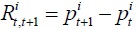 is the continuously compounded realized return between period

where  measures the speed of reversion to its fundamental value. If the estimate of
  is not observable. The other is that if

where  Note that
  is smaller than is smaller than
  4
4
2. Panel Variance Ratio Tests
We briefly present the procedure for the implementation of the panel variance ratio tests and refer to Moon and Velasco (2014) for the details. Typically, the univariate population variance ratio
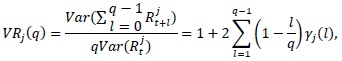
where 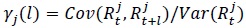 is the autocorrelation of stock return
To resolve this problem, Moon and Velasco (2014) develop an econometric method which uses information from all
Note that

They also derive a pooled variance ratio statistic: 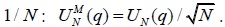 To conserve the space, we refer to Moon and Velasco (2014) for the derivation of the asymptotic distribution of
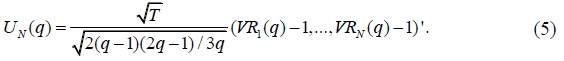
When both the time series dimension
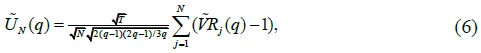
where  is calculated using defactorized series obtained from a projection of each cross section series on the cross section average return and thus to be independent standardized random variable. For deriving this statistic, they assume that cross-section dependence is due to the presence of a common factor in individual series so that defactorizing the original series can eliminate cross-section dependency. They then show that
  follows a standard Normal distribution with mean 0 and variance 1. In contrast to Richardson and Stock (1989) and Deo and Richardson (2003), this statistic still follows a standard Normal distribution even when
We use two panel variance ratio statistics,  to examine if industry group stock price indexes in Korea contain mean reverting components over long horizons. Both
  measure standardized mean variance ratios, although they are developed under different assumptions of cross-section serial dependence and the behavior of
As well known in the literature of panel unit root tests, one difficulty with the construction of panel unit root tests is how to deal with cross section dependence and heterogeneity. As shown in Moon and Velasco (2014), the asymptotic distributions of the above statistics are derived from models where cross section dependence is left completely unrestricted and does not require further modelling when
4)See, e.g.,
III. DATA
The monthly data are obtained from DataGuide for KSE (Korean Stock Exchange) and KOSDAQ (Korean Securities Dealers Automated Quotations) industry group stock price indexes.5 As explained below, we construct two samples, separately, to check robustness of our results: KSE sample and KOSDAQ sample.
The KSE sample consists of 20 KOSPI industry group stock price indexes. The listed firms in Korean Stock Exchange (or the stock market division of the Korea Exchange) have been classified into one of the industries according to Korea Standard Industry Classification. The industry groups included are as follows: Food & Beverages, Textile & Wearing Apparel, Paper & Wood, Chemicals, Medical Supplies, Non-Metallic Mineral Products, Iron & Metal Products, Machinery, Electrical & Electric Equipment, Medical & Precision Machines, Transport Equipment, Distribution, Electricity & Gas, Construction, Transport & Storage, Communications, Banks, Securities, Insurance, and Services.
On the other hand, the KOSDAQ sample consists of 18 general industry group stock price indexes and 12 IT industry group stock price indexes. We also divide the KOSDAQ sample into two subsamples, general industry group and IT industry group, to examine how the mean reversion behavior of stock prices is different between the two groups.
The industry classification in KOSDAQ industry group is different from that in KSE industry group. In particular, the former explicitly distinguishes IT industry firms from the general industry firms. Further, even for the general industry groups, the industry classification is slightly different between KSE and KOSDAQ industry groups. We separately consider these two samples to examine how the different industry classification affects the mean reverting behavior of stock returns.6
We study three sample periods: the entire sample period of 1988:02 to 2016:03, the pre Asian currency crisis period of 1988:02 to 1997:09, and the post-crisis period of 2001:01 to 2016:03. We set the beginning of the post-crisis period at 2001:01 so that we can compare the results between the KSE sample and the KOSDAQ sample more consistently. Note that the data for many of industrial stock price indexes in the KOSDAQ sample are only available since 2001, although the KOSDAQ index is available from 1997.7 We consider the two subsample periods to take into account of several factors which may affect stock price behaviors.8 First, Korean financial markets faced significant changes right after the Asian currency crisis: Korea accelerated its integration with international financial market by implementing extensive capital liberalization. According to our sample collected from DataGuide, the data for stock trades in Korea by foreign investors started to appear since 1996:02. Our sample further reveals that foreign investors actively participated in trading activity since 2000. In addition, currency crisis caused structural changes of the Korean economy in several dimensions [see e.g., Moon (2015)]. This may have affected fundamental values of stocks.
Table 1 presents some summary statistics for our sample. We calculate the averages of the number of stocks per portfolio, of annual returns, of annual Sharpe ratios, and of the ratio of market capitalization by foreign investors. For comparison, we also present relevant statistics for both KOSPI and KOSDAQ indexes.
For the KSE sample (the entire sample period of 1988-2015), the average of the number of stocks in industry-sorted portfolios is 44, the minimum number of stocks is 4 (Communications), and the maximum number of stocks is 101 (Chemicals). For the KOSDAQ sample (the sample period of 2001-2015), the average of the number of stocks in industry-sorted portfolios is 45, the minimum number of stocks is 6 (Transportation), and the maximum number of stocks is 269 (IT Hardware).
For the KSE sample, the averages of annual industrial portfolio returns are 2.97% for the entire sample period of 1988-2015, -2.57% for the pre-crisis period of 1988-1996, and 7.85% for the post-crisis period of 2001-2015. These numbers are comparable with the returns of KOSPI index: its annual returns are 2.91, -3.77, and 7.61%, respectively, for the corresponding sample periods. The average of annual industrial portfolio returns for the KOSDAQ sample is -0.03% for the post-crisis period, which is much smaller than the average portfolio rerun from the KSE sample during the same sample period. Further investigation reveals that this low return is mainly due to the bad performance of IT industry portfolios: the averages of annual industrial portfolio returns are 2.61% for the general industry groups and -3.98% for the IT industry groups in the KOSDAQ sample.
5)We also consider quarterly and yearly data to check the robustness of our results but obtain similar results (see Section IV.3).
6)This is quite conventional in the literature. For example,
7)In particular, most IT specialized companies are added to the IT industry group since 2001.
8)The results are robust with particular threshold dates: for example, we consider various dates around the currency crisis period for dividing the entire sample periods but find similar results. These results are available upon request.
IV. EMPIRICAL RESULTS
1. The KSE Sample
Figure 1 displays the results of two panel variance ratio tests,  employing monthly 20 KOSPI industry group stock returns. Panel A presents the results from the entire sample period of 1988:02-2016:03, Panel B presents those from the sample period of 1988:02-1997:09, and Panel C presents those from the sample period of 2001:01-2016:03. We set the maximum value of return horizon at
The horizontal axis represents return horizon of
We Observe the Following Results from Figure 1.
• In the entire sample period, the two variance ratios tend to stay between the two critical values.
• In the pre-crisis period,  rejects the random walk hypothesis at the left tail for most of
• In the post-crisis period, the two variance ratios tend to stay between the two critical values. Exceptionally rejects the random hypothesis at the left tail for
These results suggest that the predictability of industry stock returns is strongly detected in the pre-crisis period and significantly reduced in the post-crisis period. That is, past returns do not predict future returns in the post-crisis period, implying that the tests fail to reject the weak-form efficient market hypothesis. The third result implies that even if stock prices deviate from the fundamental value, these deviations are quickly adjusted to the fundamental value (within one year). These results are consistent with the argument that Korea’s financial markets have become more efficient since the currency crisis due to the significant integration with international financial markets and the massive amount of free capital flows.
We also find that the predictability of stock returns in the pre-crisis period is closely related to the mean reversion over long horizons. Specifically, the inversed hump-shaped pattern of is negative over almost all return horizons
2. The KOSDAQ Sample
Figure 2 displays the results of two panel variance ratio tests,  employing monthly 18 KOSDAQ general industry group stock returns as well as 12 KOSDAQ IT industry group stock returns for the sample period of 2001:01-2016:03. Panel A presents the results from the KOSDAQ sample which contains all 30 industry group stock returns, Panel B presents those from the general industry sample which only contains 18 general industry group stock returns, and Panel C presents those from the IT sample which only contains 12 IT industry group stock returns.
We observe the following results from Figure 2.
• In the KOSDAQ sample, strongly rejects the random walk hypothesis at the right tail for
• In the general industry sample, two variance ratios tend to stay between the two critical values for almost all
• In the IT sample, rejects the random hypothesis at the right tail for
These results suggest, first, that the behavior of industry stock price indexes in the KOSDAQ sample is mainly influenced by the behavior of IT industry stock price indexes. The serial dependence pattern of stock returns in the IT sample is quite similar to the KOSDAQ sample which includes both general industry and IT industry stock price indexes. Second, the serial dependence of IT industry stock price indexes is positive over most of return horizons, suggesting that stock prices do not revert to the trend even in the long run. Third, the autocorrelation pattern of general industry stock price indexes over return horizons is quite similar to that of the KSE industry stock returns during the same sample period. So, the main difference between the KOSDAQ sample and the KSE sample regarding the serial dependence pattern of stock returns comes from the behavior of IT industry stock price indexes.
3. Robustness
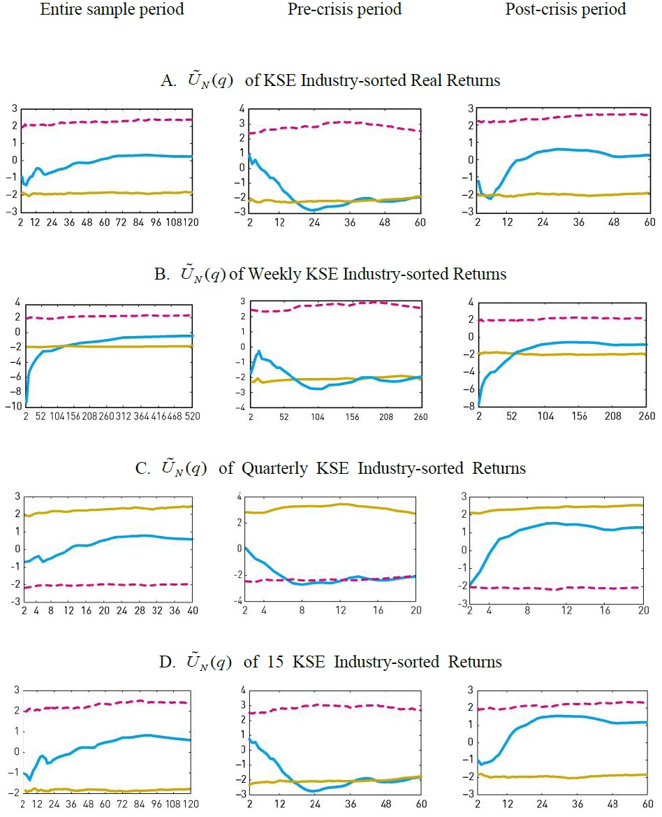
So far, we have obtained empirical results that the predictability of Korean industry group stock price indexes has been significantly reduced after the currency crisis. In this subsection, we conduct three additional exercises to check the robustness of our results: First, we replace nominal stock returns with real stock returns; second, we select different data frequencies; finally, we drop industry group portfolios which contain less than 20 firms from our sample. We discuss the results from these robust exercises one by one in detail below.
We begin with our first exercise. Although the weak-form efficient market hypothesis does not explicitly state that real or nominal stock returns are unpredictable, it may be natural to use real returns for testing it, in particular over long return horizons such as multi-year return horizons. For this, we adjust one-month continuously compounded nominal returns with the inflation rate of the Korean Consumer Price Index (CPI) and then sum to get overlapping monthly observations on longer horizon returns.
Panel A in Figure 3 displays the results of the panel variance ratio test,  for the three sample periods, employing monthly 20 KOSPI industry group real stock returns. From now on, to conserve the space, we only report the results based on and omit those based on
  We find that the results using real returns are almost identical to those using nominal returns for each of the three sample periods: like as the case of using nominal stock returns, we find significant mean reversion for the pre-crisis period and little evidence for the post-crisis period.
In the second exercises, we consider different data frequencies and use weekly or quarterly data.9 Since the efficient market hypothesis is not limited to a particular data frequency, considering various data frequencies will help us to check the robustness of the results. The use of weekly data obviously increases the size of time dimension,
Panel B and C in Figure 3 display the results of the panel variance ratio test, for the three sample periods, employing weekly and quarterly 20 KOSPI industry group stock returns, respectively. Overall, we find quite similar results to the case of using monthly data. We find significant mean reversion over long horizons for the pre-crisis period using both weekly and quarterly stock returns, consistent with the case of monthly stock returns: is much less than critical values at the 5 percentiles of the empirical bootstrap distribution for is much less than critical values at the 5 percentiles of the empirical bootstrap distribution for tends to stay between two critical values of the distribution for each
In the third exercise, we concern with a potential data snooping bias and restrict the minimum number of stocks to be included in a portfolio following Fama (1976) who argued that portfolios should contain more than 20 stocks in general to obtain gains from diversification. By applying this rule to our KSE sample, we drop three industry portfolios such as Medical & Precision Machines, Electricity & Gas, and Communications from the sample and merge three finance-related industries of Banks, Securities, and Insurance to form one industry. With this modification, the KSE sample now consists of 15 KOSPI industry group stock price indexes.
Panel D in Figure 3 displays the results of the panel variance ratio test, for the three sample periods, employing 15 KOSPI industry group stock returns. For the entire sample period and for the pre-crisis period, we find quite similar results to the benchmark case which does not restrict the minimum number of stocks in each portfolio. However, for the post-crisis period, we fail to reject the random walk hypothesis in contrast to the benchmark case: stays between the two critical values. These results further support our previous conclusion that Korean stock markets have become more efficient since the Asian currency crisis.
9)We do not consider yearly stock price data since our sample periods considered are too short.
V. CONCLUSIONS
We test the weak-form efficient market hypothesis for industry-sorted portfolios from Korean stock markets. Based on a panel variance ratio approach, we find significant mean reversion of KSE industry-sorted stock returns over long horizons in the pre Asian currency crisis period but little evidence in the post-crisis period. We also conduct several robustness checks and find that the conclusion remains unchanged. Our empirical findings are consistent with the fact that Korea accelerated its integration with international financial market by implementing extensive capital liberalization since the crisis.
Tables & Figures
Table 1.
Summary Statistics for Industrial Portfolios
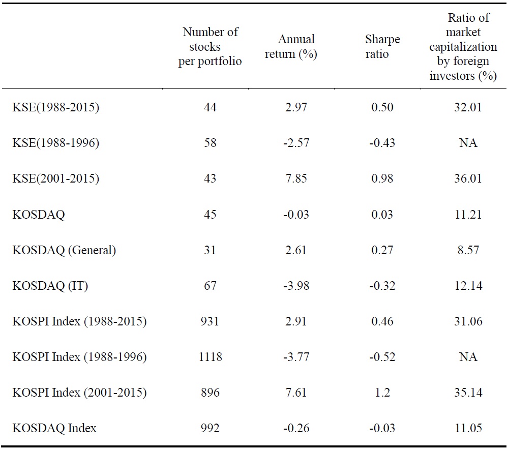
Source: DataGuide (accessed April 17th, 2016). All the numbers are the averages of industry portfolios. The numbers for KOSPI and KOSDAQ indexes are the averages over sample periods. Annual returns and Sharpe ratios are calculated using the year end of stock price indexes.
Figure 1.
Panel Variance Ratios of KSE Industry-sorted Portfolios
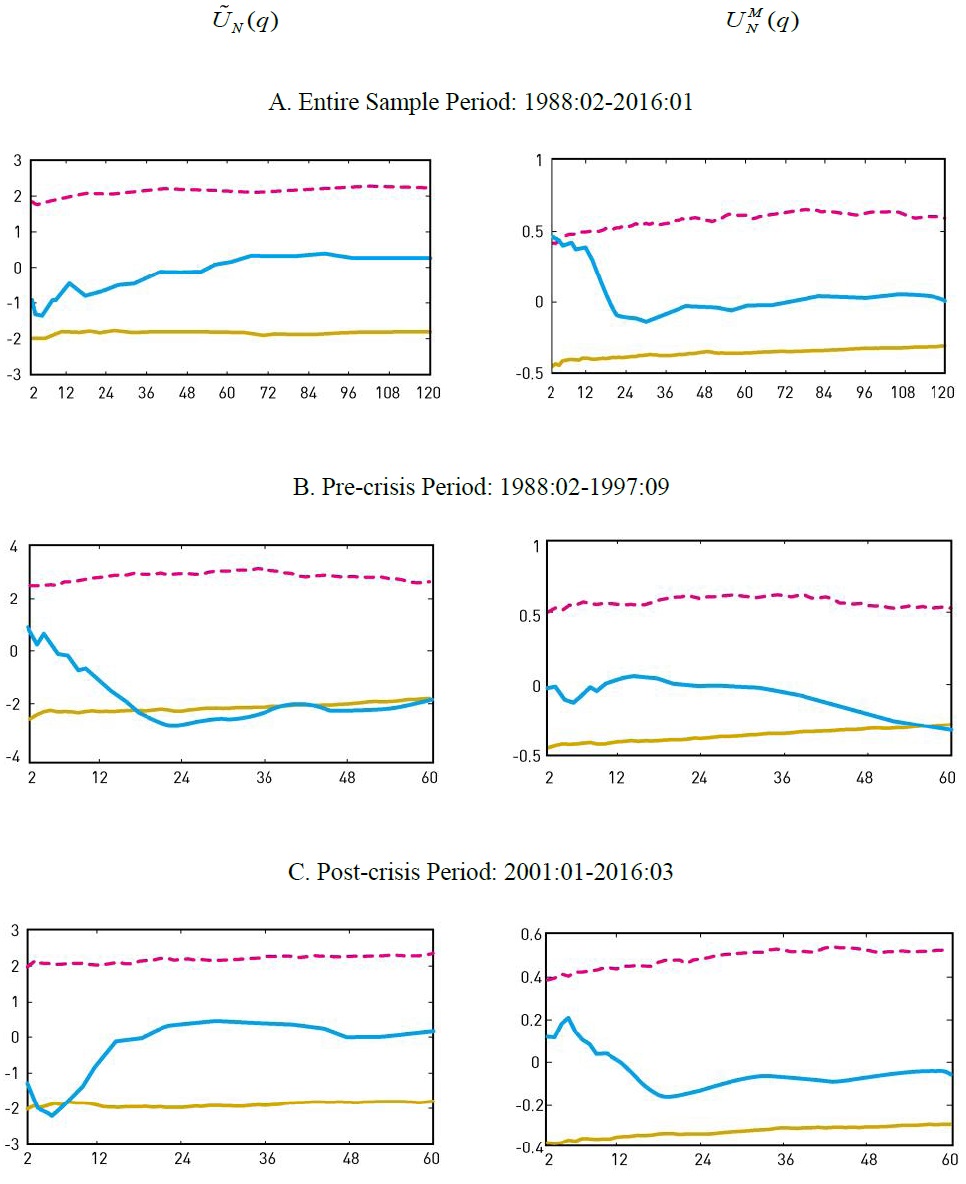
Figure 2.
Panel Variance Ratios of KOSDAQ Industry-sorted Portfolios
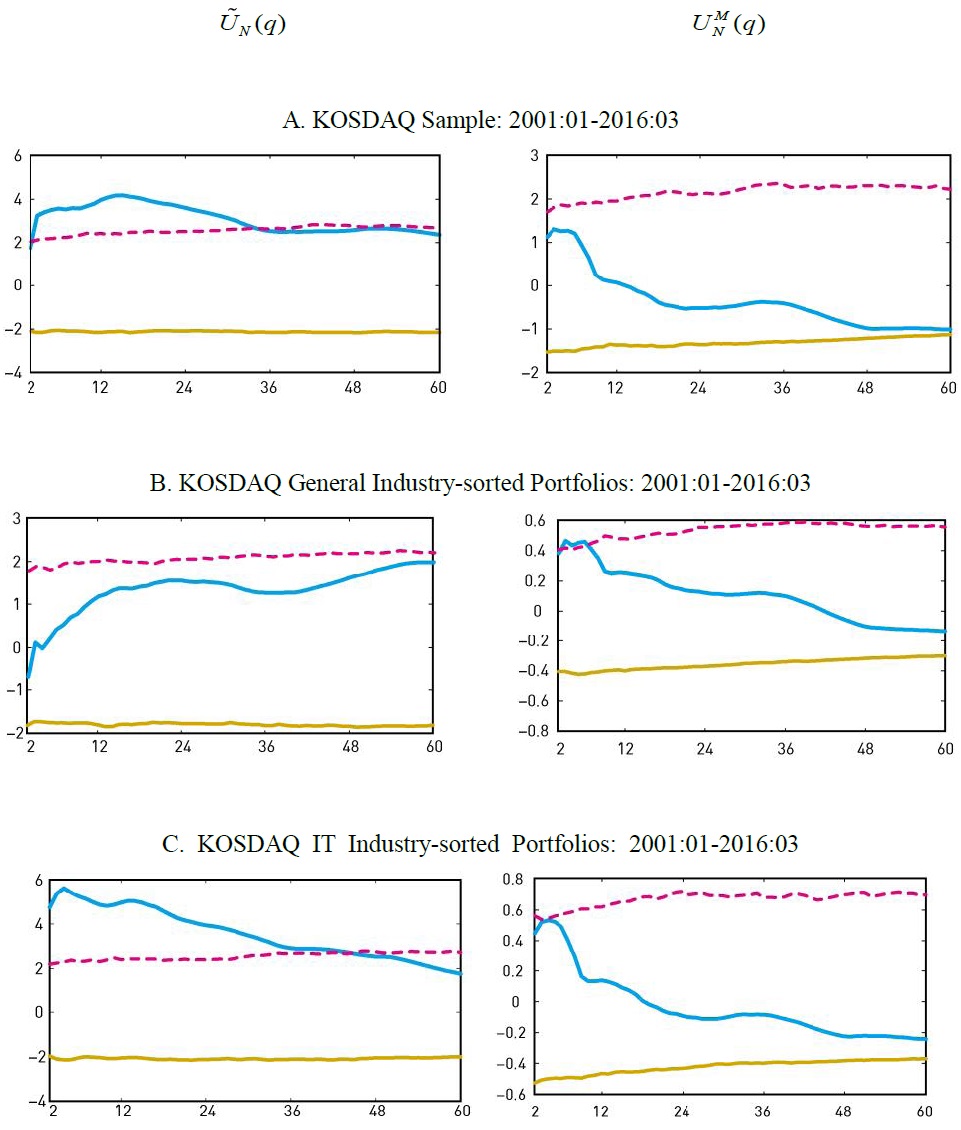
Figure 3.
Robustness Check
References
-
Bae, J. 2006. “A Reexamination of Mean Reversion and Aversion in Korean Stock Prices,”
Journal of Economic Studies , vol. 24, no. 2, pp. 85-105. (in Korean). -
Balvers, R., Wu, Y. and E. Gilliland. 2000. “Mean Reversion Across National Stock Markets and Parametric Contrarian Investment Strategies,”
Journal of Finance , vol. 55, no. 2, pp. 745 -772.
-
Campbell, J. Y., Lo, A. W. and A. C. MacKinlay. 1997.
The Econometrics of Financial Markets , Princeton, N.J. : Princeton University Press. -
Cochrane, J. H. 1988. “How Big is the Random Walk in GNP?,”
Journal of Political Economy , vol. 96, no. 5, pp. 893-920.
-
Deo, R. S. and M. Richardson. 2003, “On the Asymptotic Power of the Variance Ratio Test,”
Econometric Theory , vol.19, no. 2, pp. 231-239.
-
Fama, E. 1976.
Foundations of Finance : Portfolio Decisions and Securities Prices , New York: Basic Books. -
Fama, E. F. and K. R. French. 1988. “Permanent and Temporary Components of Stock Prices,”
Journal of Political Economy , vol. 96, no. 2, pp. 246-273.
-
Glen, J. D. 1992. “Real Exchange Rates in Short, Medium, and Long Run,”
Journal of International Economics , vol. 33, no. 1-2, pp. 147-166.
-
Gropp, J. 2004. “Mean Reversion of Industry Stock Returns in the U.S., 1926-1998,”
Journal of Empirical Finance , vol. 11, no. 4, pp.537-551.
-
Hasanov, M. 2009. “Is South Korea’s Stock Market Efficient? Evidence from a Nonlinear Unit Root Test,”
Applied Economics Letters , vol. 16, no. 2, pp. 163-167.
-
Jegadeesh, N. 1991. “Seasonality in Stock Price Mean Reversion: Evidence from the U.S. and the U. K,”
Journal of Finance , vol. 46, no. 4, pp. 1427 -1444.
-
Kapetanios, G., Shin, Y. and A. Snell. 2003. “Testing for a Unit Root in the Nonlinear STAR Framework,”
Journal of Econometrics , vol. 112, no. 2, pp. 359-379.
-
Kim, C., Nelson, C. R., and R. Startz. 1998. “Testing for Mean Reversion in Heteroskedastic Data Based on Gibbs-Sampling-Augmented Randomization,”
Journal of Empirical Finance , vol. 5, no. 2, pp. 131-154.
-
Kim, I. and C. Kim. 1999. “Korean Stock Markets, Mean Reversion or Mean Aversion,”
Kukje Kyungje Yongu , vol. 5, no. 3, pp. 97-115. (in Korean) -
Kim, M., Nelson, C. R., and R. Startz. 1991. “Mean Reversion in Stock Prices? A Reappraisal of the Empirical Evidence”
Review of Economic Studies , vol. 58, no. 3, pp. 515-528.
-
Liu, C. Y. and J. He. 1991. “A Variance-ratio Test of Random Walks in Foreign Exchange Rates”
Journal of Finance , vol. 46, no. 2, pp. 773-785.
-
Lo, A. W. and A. C. McKinlay. 1988. “Stock Market Prices Do Not Follow Random Walks: Evidence from a Simple Specification Test”
Review of Financial Studies , vol. 1, no. 1, pp. 41-66.
-
Lo, A. W. and A. C. McKinlay. 1989. “The Size and Power of the Variance Ratio Tests in Finite Samples: A Monte Carlo investigation,”
Journal of Econometrics , vol. 40, no. 2, pp. 203-238.
-
Moon, S. 2015. “Decrease in the Growth of Domestic Demand in Korea,”
Journal of East Asian Economic Integration , vol. 19, no. 4, pp. 381-408.
-
Moon, S. and C. Velasco. 2013. “Tests for M-dependence Based on Sample Splitting Methods,”
Journal of Econometrics , vol. 173, no. 2, pp. 143-159.
- Moon, S. and C. Velasco. 2014. “Panel Variance Ratio Tests,” mimeo, Universidad Carlos III de Madrid.
-
Narayan, P. K. and R. Smyth. 2004. “Is South Korea’s Stock Market Efficient?,”
Applied Economics Letters , vol. 11, no. 11, pp. 707-710.
-
Pesaran, M. H. 2007. “A Simple Unit Root Test in the Presence of Cross-section Dependence,”
Journal of Applied Econometrics , vol. 22, no. 2, pp. 265-312.
-
Poterba, J. M. and L. H. Summers. 1988. “Mean Reversion in Stock Prices: Evidence and Implications,”
Journal of Financial Economics , vol. 22, no. 1, pp. 27-59.
-
Richardson, M. and J. Stock. 1989. “Drawing Inferences from Statistics Based on Multiyear Asset Returns,”
Journal of Financial Economics , vol. 25, no. 2, pp. 323-348.
-
Summers, L. H. 1986. “Does the Stock Market Rationally Reflect Fundamental Values?,”
Journal of Finance , vol. 41, no. 3, pp. 591-601.
-
Zivot, E. and D. Andrews. 1992. “Further Evidence of the Great Crash, the Oil-price Shock and the Unit-root Hypothesis,”
Journal of Business and Economic Statistics , vol. 10, no. 3, pp. 251-270.