

- EAER>
- Journal Archive>
- Contents>
- articleView
Contents
Citation
| No | Title |
|---|
Article View
East Asian Economic Review Vol. 24, No. 3, 2020. pp. 275-301.
DOI https://dx.doi.org/10.11644/KIEP.EAER.2020.24.3.380
Number of citation : 0View
72
Download
47
Estimating State-Level Matching Efficiencies in the Indian Labor Market
|
|
Hankuk University of Foreign Studies |
|---|---|
|
|
Busan University of Foreign Studies |

Abstract
We analyze state-level matching efficiencies in the Indian labor market using stochastic frontier analysis. The key contribution of this research is the estimation of matching efficiencies at the state level because these can be used for a state-level measure of labor market conditions. Next, we explore the relationship between the estimated matching efficiencies and population density, labor market flexibility, and the Ease of Doing Business index, respectively. The results show that matching efficiency is heterogeneous across states with considerable variation in accordance with the regional diversity in India. However, we find that there is little relationship between the estimated matching efficiencies and the labor market conditions of interest, suggesting that other regional diversity affects matching efficiencies across states in India.
JEL Classification: J4, J20, J60, O53
Keywords
Matching Function, Matching Efficiency, Indian Labor Market, Stochastic Frontier Model, Population Density, Labor Market Flexibility
I. INTRODUCTION
India occupies 2.4 percent of the world’ surface area and represents 17.7 percent of the world’s population with more than 1.3 billion people, whose residence is dispersed across 29 states and 7 union territories as of 2019.1 India has huge regional diversity in terms of culture, geography, population density, and so on. There is also considerable variation in economic growth across regions (see, for example, Sachs, Bajpai, and Ramiah, 2002).
Focusing on the labor market, conditions, such as institutions, vary across regions in India. In addition to its regional diversity, there is an outstanding feature that differentiates regional achievements. In terms of labor laws, both the central and state governments have legislative power. The passage of labor legislation by the central government does not guarantee its implementation in a state. A state government can either amend or abandon the labor laws passed by the central government. Furthermore, a state government can enact its own implementation rules for laws (Gupta et al., 2009). This institutional feature makes the relative power of regional governments to the central government be distinct across regions. Therefore, these institutional forces are additional sources of substantial variation of economic outcomes across regions.
This paper estimates matching efficiencies in the job matching process in India, using state-level panel data.2 The use of the panel data is most appropriate in analyzing the Indian labor market because low labor market mobility and high variation in labor laws across states make it desirable to treat each state as an independent market (Topalova, 2007; Besley and Burgess, 2004). This paper has two main objectives. One is to estimate state-level matching efficiencies. The other is to analyze the correlations between the estimated matching efficiencies and some important attributes which could affect matching efficiency, such as population density, an index of labor market flexibility, and the Ease of Doing Business index. The estimates of matching efficiencies at the state level will provide valuable information for labor market conditions with both policy makers and businessmen to design plans to accomplish their own objectives. The estimated matching efficiencies can also complement other measures of labor market environments, such as the Ease of Doing Business ranks and an index of labor market flexibility. The correlation between matching efficiency and population density, labor market flexibility, or Ease of Doing Business warrants an interest in that this it can be compared with other countries. For example, Coles and Smith (1996) showed a positive relationship between matching efficiency and population density in Britain, suggesting that the job matching process in denser labor markets is more successful. This implies that in denser labor markets, job-seekers and employers would be closer so that they could communicate with lower search efforts. In contrast, Kano and Ohta (2005) found that there was a negative correlation between population density and matching efficiency. This could occur if firms are distributed over a wide range of standards, and job-seekers are also distributed over wide range of skill levels. In this case, matching is more difficult because a firm with high standard could possibly draw a low skilled worker.
This paper utilizes stochastic frontier models, rather than conventional estimation methods in that estimating matching efficiency is a key objective and stochastic frontier analysis is a widely used method for this purpose. Matching Efficiency is estimated by various specifications in stochastic frontier functions. The results show that matching efficiency is heterogeneous across states with considerable variation. It is also shown that the results are robust to different methods of estimating matching efficiency. It is found that the relationship between the estimated matching efficiency and other measures of labor market environment is weak. Their correlations are close to zero and not statistically significant, and thus it is suggested that a region with flexible labor market or better business conditions is not necessarily efficient in the job matching process.
This paper is organized as follows. Section 2 reviews previous studies that are relevant to this paper. Section 3 describes the data. Section 4 depicts the matching function in the framework of stochastic frontier analysis. Section 5 presents empirical results and Section 6 concludes this paper.
1)<
2)Matching efficiency indicates the ability to yield maximum matches from a given set of job-seekers and vacancies in the job matching process.
II. LITERATURE REVIEW
This section reviews three branches of literature which are related to this paper. First, since stochastic frontier model (SFM hereafter) is the main tool of our estimation, studies on SFM are briefly reviewed. Next, previous studies which analyze matching functions by SFM are introduced due to the fact that one of the main objectives is to estimate matching efficiency (ME hereafter) across regions using SFM. Lastly, since this paper estimates matching functions for India, previous studies which estimated matching functions for the Indian labor market are reviewed.
Research on SFM began in the 1970s. Starting from the seminal works by Aigner, Lovell, and Schmidt (1977) and Meeusen and van Den Broeck (1977), SFM has been popular as a subfield in econometrics as well as a standard econometric platform to estimate technical efficiency (Greene, 2008). Since these pioneering papers, a number of studies have produced many reformulations and extensions of the original SFM. A wide range of SFM can be found in Greene (2008). In addition, in-depth reviews and practical applications of SFM can also be found in Kumbhakar and Lovell (2003), Coelli et al. (2005), and Belotti et al. (2013).
The matching function is a popular tool in macro and labor economics due to its incorporation of frictions in the labor market. Pissarides (2000) supports the usefulness of the matching function in that it is not only valid in theoretical frameworks but also relevant in empirical analysis. Overall, estimation of the matching function is divided into the two approaches. The first one assumes a single labor market for a country and thus matching functions are estimated using aggregate time-series data. This approach assumes a single labor market for a country. The other is that matching functions are analyzed using disaggregated data across various dimensions (e.g., regions or industries) over time (month or year), which uses panel data. The use of panel data assumes that a national labor market is a collection of panel units such as states or industries. Early works focused on estimating the matching function itself, specifying functional forms, and testing the degree of returns to scale. Recently, scholars have gone into greater details, such as data issues and ME overtime or across regions. Petrongolo and Pissarides (2001) provide an extensive survey of empirical matching functions.
Using SFM, this paper estimates state-level ME and the relationship between ME and some labor market factors. Several studies utilize SFM in order to estimate matching functions in assessing ME, such as Ibourk et al. (2004), Kano and Ohta (2005), Fahr and Sunde (2006), Destefanis and Fonseca (2007), and Hynninen and Lahtonen (2007).
Ibourk et al. (2004) estimates matching functions for France with a panel data using SFM to identify differences in regional MEs. They found wide cross-regional differences in ME. Kano and Ohta (2005) obtain regional ME for 47 Japanese prefectures. The estimates for ME revealed substantial variations over regions. Fahr and Sunde (2006) examine ME, using panel data covering 117 regions in Western Germany. They performed SFM and found substantial variations in ME across regions. Destefanis and Fonseca (2007) use SFM to estimate the matching function and its regional efficiencies. They showed that there were huge differences in ME between the Southern and the rest of Italy.
Our paper shares some similarities to the previous studies in that it utilizes not only SFM but also panel data to estimate the matching function and its efficiency, and shows regional heterogeneities of ME across states in India. In line with Coles and Smith (1996), Ibourk et al. (2004), Kano and Ohta (2005) and Hynninen and Lahtonen (2007), our paper examines the link between population density and ME with longitudinal data.
However, in analyzing the effect of population density on matching function, most papers controlled for a proxy of population density in the matching function, which means that they added a variable for population density to a conventional specification of the matching function. Our paper differs from these papers in that state-wide regional MEs are predicted after estimation of the matching function using SFM and then the predicted values of regional ME are evaluated, by regressing ME and population density. Kano and Ohta (2005) used the same method as ours in their analysis. Our paper also investigates the link between the estimates of ME and labor market flexibility (or Ease of Doing Business index), which represents another difference from the previous studies.
Lee (2017, 2019) examines the matching function for the Indian labor market. Lee (2017) estimates the nation-wide aggregate matching function using time-series data and assessed the link between openness, as a proxy for trade liberalization, and the job matching process in this country. Lee raised a possibility that trade liberalization led to a decrease in new hires. Lee (2019) examines the role of the labor market flexibility in the job matching process in India using state-level panel data. Lee showed that there is no effect of labor market flexibility on new hires in India. However, Lee found that there are differences in the parameters of the matching functions across regions categorized by labor market flexibility.
III. DATA
1. Employment Exchange in India
Employment Exchanges in India (EEI, hereafter) are the only public employment service in India.3 EEI has a nation-wide network covering all States and Union Territories. As a public employment service in other countries, the EEI’s main role is to provide employment exchange services for job-seekers and employers as well as other services such as vocational guidance, career counseling, and special services for the handicapped (DGE&T, 2018)
As of December 31, 2017, EEI had 997 offices, covering 28 states and 7 union territories.4 Among the 997 offices, 80 offices specialized in employment for physically handicapped, 76 offices were bureaus for university students seeking employment, 14 offices served executives and other professionals, and 5 offices were exclusively for women (DGE&T, 2018).
In addition to its job matching and other services, the EEI collects raw data on employment, unemployment and other information that are relevant to policy planning and research (DGE&T 2018, p. 1). Labor market information in India collected by the EEI includes details on gender, minorities, handicapped, age, education level, immigrants, and regions (DGE&T, 2018). Each state’s EEI offices collect a variety of data at the district or state level and the Directorate General of Employment and Training (hereafter DGE&T) at the Ministry of Labour and Employment puts together and publishes the data at the national level (DGE&T 2018, p. 1).5 Employment Directorate in the DGE&T assesses and observes employment and unemployment situation over all levels in India using various sources such as Census, Labour Force Surveys conducted by National Sample Survey Organisation and Employment Market Information Programme and so forth.
The data used in this paper is drawn from various
2. Data Description
The variables in the matching function correspond to the measures in
The cross-section unit is a State or a Union Territory and total number of panel units is 34. Two panel units are omitted in this study. One is Telangana, previously belonging to Andhra Pradesh, as it became the 29th state of India in June 2014. The other region is Sikkim, where there is no EEI office. In the original dataset, the data are available from 1999 to 2017 but not stable from 2014 to 2017. There are missing values for the main variables in 9 states. For example, Delhi’s data for
This paper incorporates three more variables, population density (PD hereafter), labor market flexibility (LMF hereafter), and the Ease of Doing Business index (EDB hereafter) in its analysis. PD is a measure of population per unit area. The latest data of PD over states in India is available from the Population Census 2011.7 The Census of India provides population per square kilometer in each state in 2011. There are several measures of LMF in India. The OECD’s index for employment protection legislation is utilized as an indicator of LMF (OECD, 2007). The LMF indicates the degree of LMF for the 21 states in terms of variations in implementing and administrating labor laws across states (Dougherty et al., 2011). Although only LMFs of 21 states are available, the information from these states is meaningful because these 21 states account for 98 percent of both the GDP and the population in India (OECD 2007, p. 139). To measure overall labor market rigidity, the OECD survey covers not only the Industrial Dispute Act, but also other major labor laws including the Factories Act, the State Shops and Commercial Establishment Acts, the Contract Labor Act, the role of inspectors, the maintenance of registers, the filing of returns and union representation (Dougherty et al. 2011, p. 13). In fact, OECD’s LMF is a modified version of Besley and Burgess (2004). However, the reason to use the OECD’s data is that Besley and Burgess covers less number of states than the OECD’s index (21 states by OECD and 15 states by Besley and Burgess) and their index is constructed by using the Industrial Dispute Act only.
The EDB is measured by the World Bank. Its annual publication,
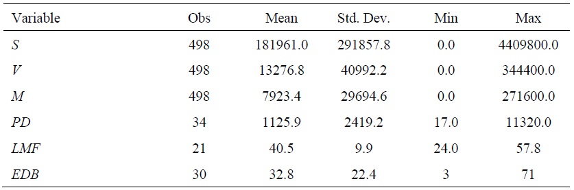
Table 1 provides the descriptive statistics for the variables used in this paper. The average of the number of job-seekers across 34 states and over 15 years was 181,961, whereas the averages for job vacancies and job placements were 13,276 and 7,923, respectively. These numbers indicate a lack of job vacancies, which implies a dependence on labor demand in the job matching process, before incorporating heterogeneities across states. Higher standard deviations of vacancies and placements also show larger variations in these variables. Especially, a high variation in placements displays different level of matching frictions across states. PD also shows substantial variation across states, which is confirmed by much larger value of standard deviation than average.
Figure 1 shows the annual trends of job-seekers, vacancies, and placements. The trends of vacancies and placements look similar over time. These two trends declined until 2002, but recovered from 2003. The increase in 2003 is consistent with India’s spur in its growth, starting from 2003. The downturn in 2009 and declines in 2012 and 2013 were due to world-wide economic crisis and recessions. With the exception of 2006 and 2012, the number of job-seekers did not show significant fluctuation.
3)Public employment service is a governmental organization and its main objective is to link job-seekers and businesses.
4)As of 2017, there is no EEI office in Sikkim, a state in India.
5)The State and Union territorial governments exercise administrative and financial authority over the respective EEI offices
6)India’s fiscal year is from April 1 to March 31.
7)<
8)
9)
IV. SPECIFICATION OF A MATCHING FUNCTION IN THE STOCHASTIC FRONTIER FRAMEWORK
The job matching process between job-seekers and employers is costly in terms of time and effort, due to search frictions including exchange friction, imperfect information, and individual heterogeneity. Matching function summarizes these underlying search frictions and matching process in the labor market. It is simply depicted by the joint movement of job-seekers and vacancies to create job placements. Its general form is given as
In estimating efficiency of the matching function, like that of the production function, it is assumed that the matching process yields maximum feasible matches for a given level of job-seekers and vacancies but potentially can produce less than it might be due to a certain degree of inefficiency.10 SFM formulates that observed deviations from the matching function are caused by two factors: matching inefficiency and idiosyncratic random effects. Thus, the matching function with idiosyncratic error and a degree of inefficiency is defined as Equation (1):

Since Cobb-Douglas specification is a widely used functional form of the matching function (Petrongolo and Pissarides, 2001), assuming Cobb-Douglas functional form and taking the natural logarithm of the both sides of Equation (1) yield:

Defining that

The
It is assumed that
ME can be defined as the ratio of observed matches to stochastic frontier matches in Equation (4):

It is the most desirable to estimate  where
where 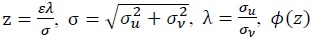 is pdf of the normal distribution, and
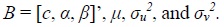
Maximum likelihood estimation (MLE) based on Equation (3) is used to estimate these parameters. A time-invariant ME’s case,
The common feature of the above specifications, either time-invariant or timevarying, is that SFMs’ intercept,

The intercept term in Equation (3) is replaced by
10)Given a certain quantity of inputs (S and V), ME is achieved when the maximum new hires (M) are generated. Thus, it is said that ME is higher if higher matches are generated, given S and V. ME is important measure due to the fact that it shows a performance of the job matching process.
V. ESTIMATION RESULTS
One of the problems in EEI data is that the data is unrepresentative of the Indian labor market. Figure 2 presents marked differences in the distributions of job-seekers and the population across States and Union Territories. For instance, the population share in Uttar Pradesh is the largest, while the job-seekers’ proportion of Tamil Nadu is the highest in terms of the number of job-seekers through EEI. This disproportionality may influence the representativeness of the sample. To deal with this issue, regression analysis of all specifications in this paper is performed using the population distribution in Figure 2 as a sampling weight.
The other issue is endogeneity. In estimation of the matching function, an endogeneity problem arises when the flow variables are estimated as a function of the stock variables (Petrongolo and Pissarides, 2001). Data for the number of job placements,
One noticeable advantage of using the data in this paper is that its panel unit is a state. Hasan et al. (2012, p. 270) argue that each state in India has its own authority over economic issues, especially in labor legislation, and thus, state-level analysis is suitable for analyzing the Indian labor market. Hasan et al. also suggest that it is reasonable to count each state as an independent labor market on the basis of low labor mobility and variations in labor institutions across states (Topalova, 2007; Besley and Burgess, 2004).11
1. Estimation of Matching Functions
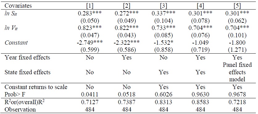
Before estimating ME of individual state, matching functions are estimated using OLS (Ordinary Least Squares), LSDV (Least Squares Dummy Variable) and panel regression methods, as shown in Table 2. Column [1] provides the results obtained by controlling for job-seekers and vacant jobs only. Column [2] gives the estimates by adding year-fixed effects to [1]. Column [3] shows the estimates by adding state-fixed effects but dropping year-fixed effects. Column [5] presents the results from performing fixed-effects panel regression with year-fixed effects. Random-effects panel regression was also performed but the result from the Hausman test is in favor of fixed-effects against random-effects. Thus, only the results from fixed-effects model are reported. The findings of [1] to [4] demonstrate the importance of heterogeneities across states. There are significant changes in the coefficients for job-seekers and job vacancies after controlling for state-fixed effects. Although addition of year-fixed effects affects the estimates for job-seekers and vacant jobs, it is not substantial. The coefficients for job-seekers and vacancies after controlling for state-wide heterogeneities and time effects show that the elasticities of job placements with respect to job-seekers and job vacancies are approximately 0.30 and 0.70, respectively. These estimates imply that the contribution of vacancies is higher than that of job-seekers. This can also be interpreted as a relative shortage of labor demand. When state-fixed effects are controlled, the constant returns to scale of the matching function is not rejected, as shown in Columns [3], [4], and [5]. This result is in accordance with a number of previous studies (e.g., Petrongolo and Pissarides, 2001).12
2. Estimation of Stochastic Frontier Models to Produce Matching Efficiencies across States
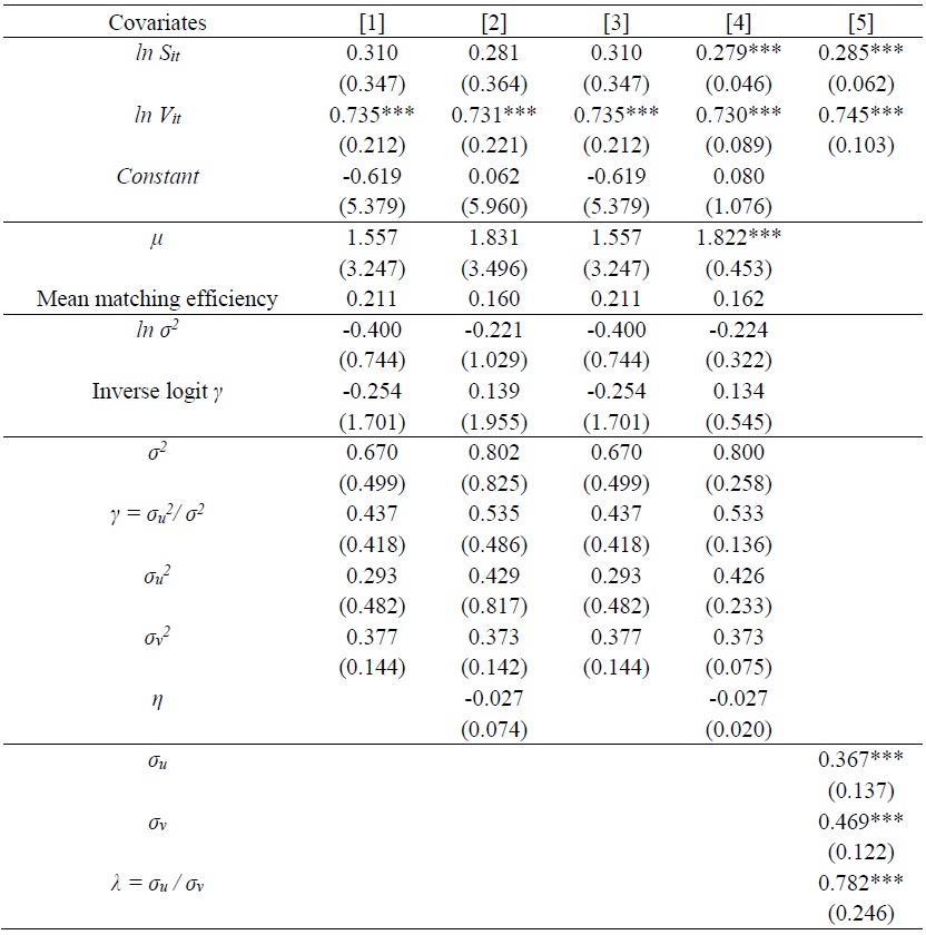
The key objective in this paper is to estimate the degree of efficiency of the matching process across states. To obtain the robustness of the estimation, MEs were estimated by various estimation methods. Table 3 presents the results from estimating matching functions using SFMs. Column [1] displays the results from performing a SFM with time invariant ME. The inefficiency term is assumed to be 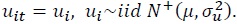 13 Column [2] presents the estimates and related information using a SFM with time varying decay model by Battese and Coelli (1992). The matching inefficiency is designed as
 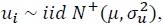 and
and
Coefficient estimates for job-seekers and vacancies in Table 3 look similar to the estimates in Table 2, although there are slight differences. Overall, the estimates for job-seekers and vacancies are approximately 0.30 and 0.70. The other disparity of coefficients between Tables 2 and 3 is that in case of [1], [2], and [3] in Table 3, i.e., without heteroscedastic robust standard errors, the estimates for job-seekers are not statistically significant.
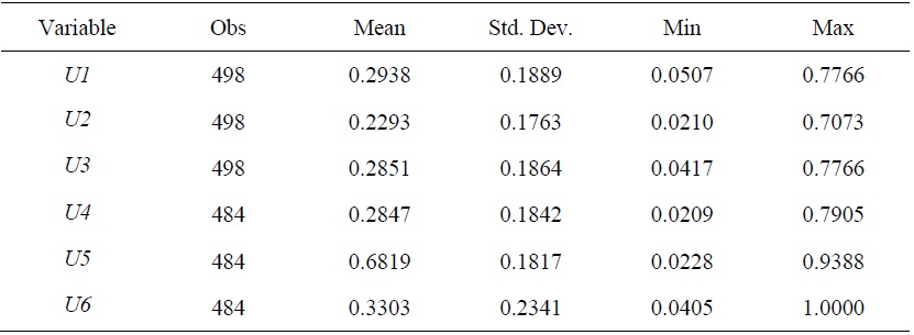
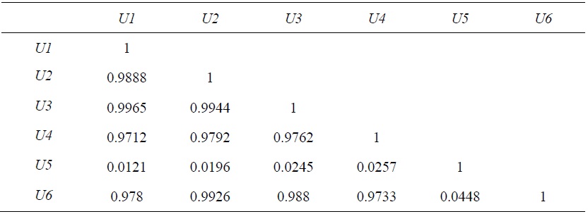
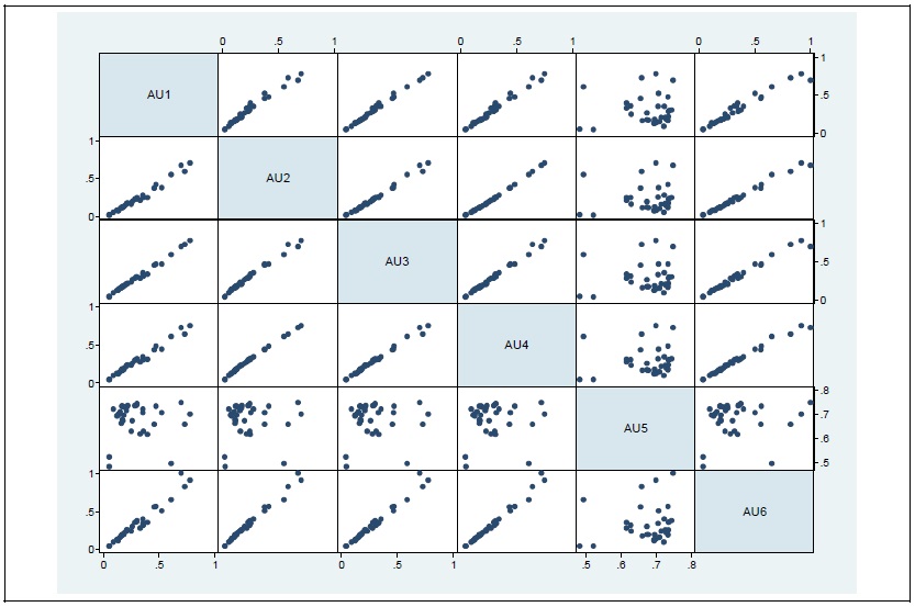
As mentioned in the previous section, the central reason to employ SFM is to estimate the disturbance of ME. Hence, the next step is to generate estimates of ME. Table 4 presents summary statistics of the ME estimates and Table 5 shows correlations of ME estimates, obtained by various SFMs. In Tables 4 and 5, one more measure of ME (Cornwell et al., 1990) is added. Cornwell et al. used a standard panel fixed-effects regression to estimate technical inefficiency (same as [5] in Table 2). They performed panel fixed-effects regression, and computed mean values of the disturbance for each panel unit over time to yield time invariant disturbance for each  where
where  .14
.14
Table 4 shows that the mean value of
The estimates of ME in different methods reveal their similarity except the estimates from TFEs by Greene (2005). There are two main disparities between TFEs and other SFMs. First, regular SFMs open a possibility of time-invariant ME but true fixed effects model strictly impose time-varying efficiency of the matching. But TFEs model disentangles regional fixed-effects from ME, whereas other stochastic frontiers’ efficiency is obtained without dealing with a region’s intrinsic effects.
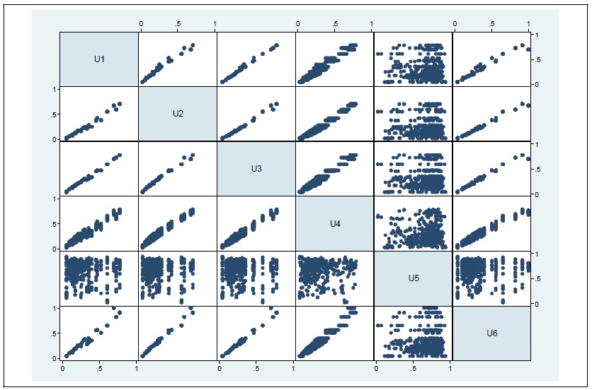
When all values for ME are averaged over time, summary statistics and correlation do not change much, compared those derived from all observations. Table 6, Table 7 and Figure 4 confirm this similarity of MEs.
Since all MEs, except
3. Relationship between Matching Efficiencies and Variables of Interest
It is shown that basic statistics of MEs (mean, standard deviation, maximum and minimum values) as well as correlations among MEs did not change much when the estimates of MEs are aggregated over time to produce time-invariant state-level MEs. The reason to aggregate MEs over time is that the estimates from standard SFMs tend to be time-invariant. The other reason is that the variables of interest are only available as time-invariant data or are available for selected years. The index for LMF created by OECD (2007) is time invariant. For PD, only decennial data are available and the latest one is the data in 2011. In EDB’s case, state level measures are only available for 2015.
In this section,
Table 8 presents the results from the second stage estimation to examine the relationships between ME and three key variables, respectively.15 The results show that the relationship between ME and PD reveals minimal or no statistical significance. Moreover, its economic effect is very small. The estimates for LMF and EDB also show little economic impact as well as no statistical significance. These findings contradict either positive or negative relationship between ME and PD. The positive relationship implies that a region with higher PD would more efficiently absorb job-seekers and job vacancies (e.g., Coles and Smith, 1996). In contrast, the negative relationship means that higher PD decreases ME in a region, which claims that the ME is negatively related to the degree of conflicts among employers’ hiring standards and worker’s skill level (Kano and Ohta, 2005). This negative relationship implies that job matching between job-seekers and businesses is more difficult if firms are distributed over a wide range of standards, due to the possibility that a firm with high standard draws a low-skilled worker. The findings on LMF are consistent with Lee (2019), showing that when LMF was added to the matching function, its coefficient estimate is small and not statistically significant, which implies that there is no additional increase in new job placements by LMF in the job matching process. Weak correlation between ME and PD, ME and LMF, or ME and EDB indicates that other factors may be more important elements affecting ME in India than the well-known factors of PD, LMF, and EDB in other countries. Each State in India has its own power over economic issues. Moreover, there are regional differences due to cultural, religious, ethnic, and other factors.
11)Low labor mobility across regions is a desirable condition in analyzing labor market outcomes with the use of state-level data. If labor mobility across states is free, then labor supply increases in states with lower labor market flexibility (for example due to higher minimum wage) due to the fact that workers in other states tend to move to regions with lower level of labor market flexibility. This can result in more labor supply than labor demand, which represents a relative shortage of labor demand.
12)Constant returns to scale (CRS) of the matching function in search-matching model implies the existence of a unique stable unemployment. In practice, CRS also implies that job placements does not depend on the absolute size of job-seekers and job vacancies but the relative size of job-seekers with respect to job vacancies or vice versa.
13)Other distributions of matching efficiency such as exponential and gamma distributions are also used. More importantly, various functional forms of matching efficiency are utilized in estimating matching efficiencies. The estimates from various distributions and functional forms of matching efficiency, however, were not different from the estimates in this paper.
14)
15)In this paper, only labor market related variables are considered. Therefore, other interesting variables, e.g., economic growth rates across states, are not included in the analysis.
VI. CONCLUDING REMARKS
In this paper, the state-level matching efficiencies in the Indian labor market are estimated using stochastic frontier models. The correlation between the estimated matching efficiency and population density, labor market flexibility, or the Ease of Doing Business index is also evaluated, respectively. It is shown that the estimates for matching efficiency reveal a considerable variation across states. However, no relationship is found between matching efficiency and the factors of interest. The absence of a relationship between matching efficiency and labor market conditions shows that other factors affect matching efficiency in India: each state has its own authority over a number of institutional issues such as labor legislation. More importantly, India’s diversity of culture, religion, and ethnicity contributes to regional differences in matching efficiency across regions.
This paper’s main contribution is that it introduces an additional measure of labor market conditions or business environment across states in India. Similar to the index of labor market flexibility from the OECD and ranks of investment environment from the World Bank’s Doing Business index, the state-wide estimates of matching efficiency can also be referred as an index for state-level information in the Indian labor market. In addition, the measure of matching efficiency covers more regions than labor market flexibility and the Ease of Doing Business index and this is also a contribution of our research to study the labor market in India.
The disparity should be clarified by analysis of the relationship between matching efficiency and population density among previous studies and this paper. This paper and Kano and Ohta (2005) estimated matching efficiency across regions in the first stage and then with new estimates of matching efficiency, the relationship between matching efficiency and population density is analyzed in the second stage of regression analysis, while Coles and Smith (1996), Ibourk et al. (2004), Hynninen and Lahtonen (2007), and others controlled the variable of population density in the first stage, in estimation of conventional matching functions. Therefore, the results from the latter studies should be interpreted as an additional effect of population density on new hires or matches in the job matching process, after controlling for job-seekers, job vacancies, and other basic factors such as time- and region-specific effects.
A point to be noticed is that this research only focuses on the link between matching efficiency and labor market conditions. To suggest more desirable policy implications, further research to incorporate key economic variables, such as economic growth, should be performed.
Tables & Figures
Table 1.
Descriptive Statistics of the Variables
Notes:
Source:
Figure 1.
Annual Trends of Job-Seekers, Job Vacancies, and Job Placements
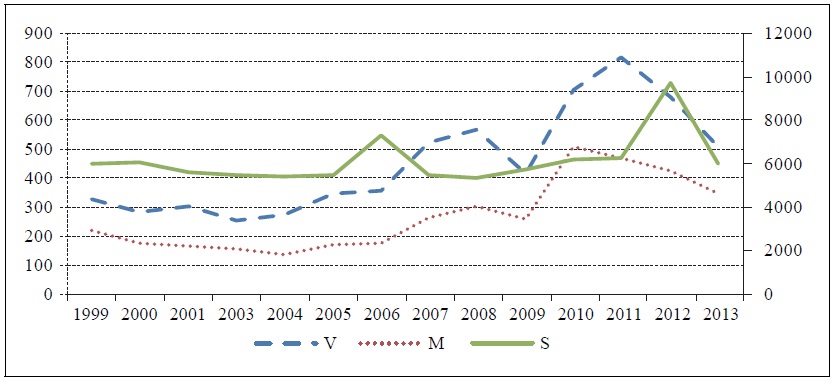
Note: The unit is thousand. The left axis is for V and M and the right axis is for S.
Source: DGE&T (2000 - 2014)
Figure 2.
Comparison between Job-seekers’ share and Population Share by State
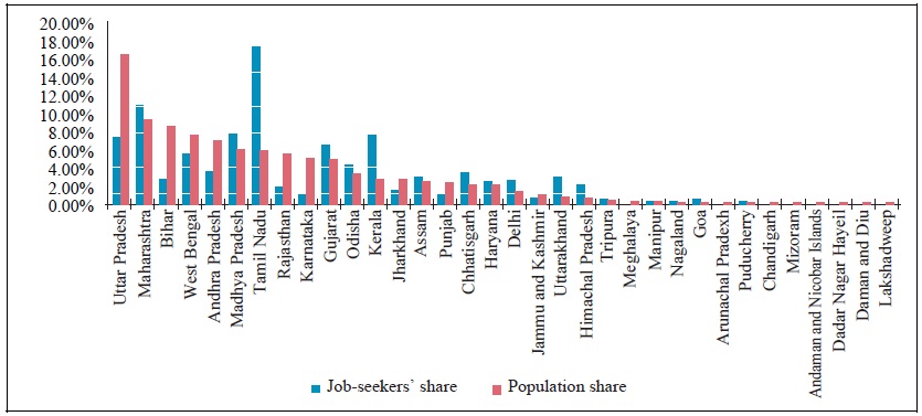
Note: Job-seekers’ share is the number of job-seekers in a state divided by total number of job-seekers in India through EEI in 2011. Population share is the population share by state in 2011.
Source:
Table 2.
OLS and Panel Regression (Dependent variable =
Notes:
Table 3.
Stochastic Frontier Models (Dependent variable =
Notes:
Table 4.
Summary Statistics for Efficiency Estimates (all sample)
Note:
Table 5.
Correlation of Efficiency Estimates (all sample)
Note: Regarding variable description, see
Figure 3.
Pairwise Scatterplots of MEs (all sample)
Note: Regarding variable description, see
Table 6.
Summary Statistics for Efficiency Estimates (state average)
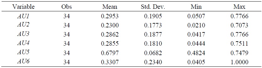
Notes:
Table 7.
Correlation of Efficiency Estimates (state average)
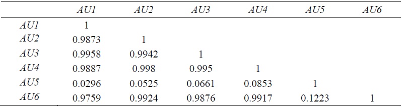
Note: Regarding variable description, see
Figure 4.
Pairwise Scatterplots of MEs (state average)
Note: Regarding variable description, see
Figure 5.
Regional Differences in Matching Efficiency
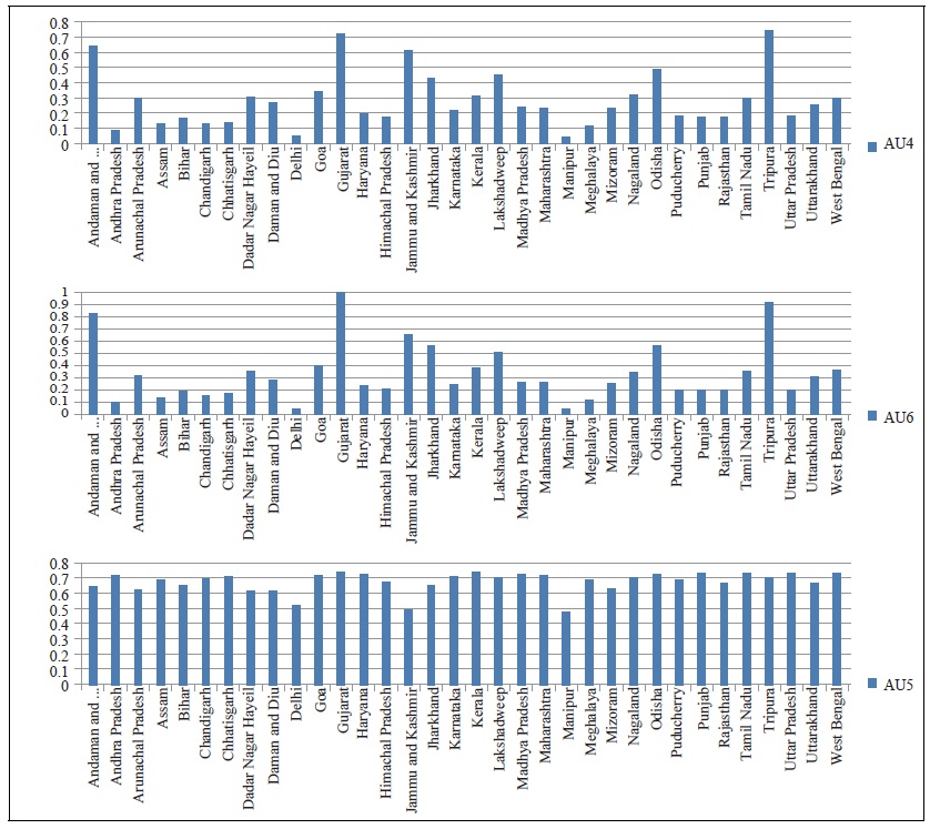
Table 8.
Relationship between ME and variables of Interest
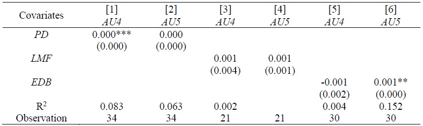
Note: Standard errors in parenthesis are robust standard errors.
References
-
Aigner, D., C. A. Knox Lovell, K. C. A. and P. Schmidt. 1977. “Formulation and Estimation of Stochastic Frontier Production Function Models,”
Journal of Econometrics , vol. 6, no. 1, pp. 21-37. -
Battese, G. E. and T. J. Coelli. 1992. “Frontier Production Functions, Technical Efficiency and Panel Data: with Application to Paddy Farmers in India,”
Journal of Productivity Analysis , vol. 3, pp. 153-169.
-
Belotti, F., Daidone, S., Ilardi, G. and V. Atella. 2013. “Stochastic Frontier Analysis Using Stata,”
Stata Journal , vol. 13, no. 4, pp. 719-758.
-
Besley, T. and R. Burgess. 2004. “Can Labor Regulation Hinder Economic Performance? Evidence from India,”
Quarterly Journal of Economics , vol. 119, no. 1, pp. 91-134.
-
Bhattacharya, A., Bruce, A. and S. Agrawal. 2015.
Future of Indian Manufacturing: Bridging the Gap . Mumbai: Boston Consulting Group. -
Coelli, T. J., Rao, D. S. P., O’Donnell, C. J. and G. E. Battese. 2005.
An Introduction to Efficiency and Productivity Analysis . New York: Springer Science & Business Media. -
Coles, M. G. and E. Smith. 1996. “Cross-Section Estimation of the Matching Function: Evidence from England and Wales,”
Economica , vol. 63, no. 252. pp. 589-597.
-
Cornwell, C., Schmidt, P. and R. C. Sickles. 1990. “Production Frontiers with Cross-Sectional and Time-Series Variation in Efficiency Levels,”
Journal of Econometrics , vol. 46, nos. 1-2, pp. 185-200.
-
Destefanis, S. and R. Fonseca. 2007. “Matching Efficiency and Labour Market Reform in Italy: A Macroeconometric Assessment,”
Labour , vol. 21, no. 1, pp. 57-84.
- Directorate General of Employment & Training (DGE&T). 2018, Employment Exchange Statistics 2018. and previous publications. New Delhi: Ministry of Labour and Employment, Government of India.
- Dougherty, S., Robles, V. F. and K. Krishna. 2011. Employment Protection Legislation and Plant-Level Productivity in India. OECD Economic Department Working Papers, no. 917.
-
Fahr, R. and U. Sunde. 2006. “Regional Dependencies in Job Creation: An Efficiency Analysis for Western Germany,”
Applied Economics , vol. 38, no. 10, pp. 1193-1206.
-
Greene, W. H. 2003.
Econometric Analysis . 5th ed. Upper Saddle River, NJ: Prentice Hall. -
Greene, W. H. 2005. “Reconsidering Heterogeneity in Panel Data Estimators of the Stochastic Frontier Model,”
Journal of Econometrics , vol. 126, no. 2, pp. 269-303.
-
Greene, W. H. 2008. “The Econometric Approach to Efficiency Analysis.” In Fried, H. O., Lovell, C. A. K. and S. S. Schmidt. (eds.)
The Measurement of Productive Efficiency and Productivity Growth . New York: Oxford University Press. pp, 92-250. -
Gupta, P., Hasan, R. and U. Kumar. 2008/2009. “Big Reforms But Small Payoffs: Explaining the Weak Record of Growth in Indian Manufacturing,”
India Policy Forum , vol. 5, no. 1, pp. 59-123. -
Hasan, R., Mitra, D., Ranjan. P. and R. N. Ahsan. 2012. “Trade Liberalization and Unemployment: Theory and Evidence from India,”
Journal of Development Economics , vol. 97, no. 2, pp. 269-280.
-
Hynninen, S.-M. and J. Lahtonen. 2007. “Does Population Density Matter in the Process of Matching Heterogeneous Job Seekers and Vacancies?”
Empirica , vol. 34, no. 5, pp. 397-410.
-
Ibourk, A., Maillard, B., Perelman, S. and H. R. Sneessens. 2004. “Aggregate Matching Efficiency: A Stochastic Production Frontier Approach, France 1990–1994,”
Empirica , vol. 31, no. 1, pp. 1-25.
-
Jondrow, J., Lovell, C. K., Materov, I. S. and P. Schmidt. 1982. “On the Estimation of Technical Inefficiency in the Stochastic Frontier Production Function Model,”
Journal of econometrics , vol. 19, nos. 2-3, pp. 233-238.
-
Kano, S. and M. Ohta. 2005. “Estimating A Matching Function and Regional Matching Efficiencies: Japanese Panel Data for 1973-1999,”
Japan and the World Economy , vol. 17, no. 1, pp. 25-41. -
Kumbhakar, S. C. and C. A. K. Lovell. 2003.
Stochastic Frontier Analysis . Cambridge University Press. -
Kumbhakar, S. C., Wang, H.-J. and A. Horncastle. 2015.
A Practitioner’s Guide to Stochastic Frontier Analysis Using Stata . New York: Cambridge University Press. -
Lee, W. 2017. “Trade Liberalization and the Aggregate Matching Function in India,”
Asian Economic Papers , vol. 16, no. 1, pp. 120-137.
-
Lee, W. 2019. “The Role of Labor Market Flexibility in the Job Matching Process in India: An Analysis of the Matching Function Using State-Level Panel Data,”
Emerging Markets Finance and Trade , vol. 55, no. 4, pp. 934-949.
- Mastromarco, C. 2008. Stochastic Frontier Models. Research Paper, Department of Economics and Mathematics-Statistics, University of Salento.
-
Meeusen, W. and J. van Den Broeck. 1977. “Efficiency Estimation from Cobb-Douglas Production Functions with Composed Error,”
International economic review , vol. 18, no. 2, pp. 435-444.
-
Organisation for Economic Co-operation and Development (OECD). 2007.
OECD Economic Survey of India . Paris: OECE Publishing. -
Petrongolo, B. and C. A. Pissarides. 2001. “Looking into the Black Box: A Survey of the Matching Function,”
Journal of Economic literature , vol. 39, no. 2, pp. 390-431.
-
Pissarides, C. A. 2000.
Equilibrium Unemployment Theory . 2nd edition, Cambridge, Mass. : MIT press. -
Population Census 2011. <
http://www.census2011.co.in/density.php > (accessed May 21, 2020) -
Sachs, J. D., Bajpai, N. and A. Ramiah. 2002. “Understanding Regional Economic Growth in India,”
Asian Economic Papers , vol. 1, no. 3, pp. 32-62.
-
Topalova, P. 2007. “Trade Liberalization, Poverty and Inequality: Evidence from Indian Districts.” In Harrison, A. (ed.)
Globalization and Poverty . Chicago: University of Chicago Press. pp. 291-336. -
World Bank. 2020.
Doing Business 2020 . Washington: World Bank Publishing. -
World Bank Open Data. <
https://data.worldbank.org > (accessed May 21, 2020)