

- EAER>
- Journal Archive>
- Contents>
- articleView
Contents
Citation
| No | Title |
|---|
Article View
East Asian Economic Review Vol. 28, No. 2, 2024. pp. 245-273.
DOI https://dx.doi.org/10.11644/KIEP.EAER.2024.28.2.436
Number of citation : 0View
46
Download
22
Limited Financial Market Participations and Shocks in Business Cycles in Korea
|
|
Kyung Hee University |
|---|

Abstract
This paper sets up a small open new Keynesian economy model with constrained households and incomplete markets to address the driving forces of business cycles in Korea. It shows that there exists a substantial fraction of constrained households who cannot have access to financial market. Furthermore, the estimated model reveals that a TANK model is better than a RANK model in explaining business cycles in Korea. The effect of domestic productivity shock on Korean economy has dominated in the variations of output, while the contribution of the foreign productivity shock to the variations of output and inflation has increased after the Asian financial crisis. The monetary policy shock has dominated the variation of inflation at short and medium horizons.
JEL Classification: E32
Keywords
Business Cycles, HtM, Korea, Maximum Likelihood Estimation, TANK
I. Introduction
A burgeoning of literature on the heterogeneous agent New Keynesian (HANK) model has contributed to understanding the transmission of monetary and fiscal policy over the business cycle. Market incompleteness and heterogeneity have been utilized to address the interaction between inequality and fiscal and monetary policy. Kaplan et al. (2018) show that the general equilibrium effect of an interest rate cut, operating through an increase of household income associated with the labor demand expansion, dominates the direct effect associated with the intertemporal substitution. Auclert et al. (2019) argue that the fiscal multipliers depend on the interaction of an intertemporal marginal propensity to consume, i.e., iMPC and deficit-financed fiscal policy and only the HANK model can generate the empirical iMPC. McKay et al. (2016) address how the HANK model can solve the forward guidance puzzle arising from the representative agent new Keynesian (RANK hereafter) model.
The quantitative HANK models that explicitly take into account heterogeneity and the feedback effects from equilibrium distributions to aggregates are successful in delivering the general equilibrium effect of exogenous shocks comparable to the one in the data. However, it is difficult to track the wealth distribution, as it is necessary to use nontrivial computational techniques to solve the equilibrium in the HANK models.
The earlier literature on two-agent models to address the business cycle has emphasized the heterogeneity in shaping the transmission of monetary and fiscal policy. The two-agent new Keynesian (TANK) model with a minimal heterogeneity and analytical tractability has been utilized to understand and quantify the implications of heterogeneity in households. In the canonical TANK model, there is a constant fraction of constrained or hand-to-mouth (HtM hereafter) households who cannot have access to the financial market and have to consume their current income. Other fraction of households, called unconstrained or Ricardian households who can have access to financial market satisfy the Euler equation. Though the simple TANK model does not allow any idiosyncratic shock and endogenous fraction of constrained households, Debortoli and Galí (2019) show that the tractable TANK model can approximate the dynamics of the HANK model under comparable redistribution schemes.1
The open economy TANK model is isomorphic to the open economy representative agent new Keynesian (RANK) model. However, there are stark differences between a TANK model and a RANK model in open economy. First, the aggregate demand equation, i.e., the unconstrained household’s Euler equation in the TANK model is different from the one in the RANK model in that the former depends on the aggregate demand as well as the fraction of HtM households in the economy. Second, only consumption of unconstrained households matters to the risk-sharing in an open economy as HtM households cannot participate in financial markets. Finally, the NKPC and goods market clearing condition depends on consumption and income inequality between unconstrained households and HtM households.
The question about the important role of financial frictions in shaping the business cycle in Korea has been actively debated in Korean academia and policy makers since the Korean government has adopted an export driven economic growth strategy from the 1960s. Some critics have been skeptical about the sustainability of the economic growth strategy in Korea where a substantial fraction of economically neglected households exists. They have criticized the structure of the Korean economy, since the economy which heavily depends on the rest of the world is too fragile to sustain its stable economic growth.
In this paper, we address the following questions with a TANK model with incomplete markets. How important have the economically neglected households, i.e., the HtM households been in shaping the business cycle in Korea over time? Specifically, does the TANK model perform better than the RANK model in explaining business cycles in Korea? What kind of shock has been the main driving force in business cycles in Korea? What fraction of HtM households have been in Korea? Has the fraction of HtM households who cannot have access to financial markets increased in Korea over time during 1997 Asian financial crisis and the ongoing Great Moderation periods?
For this purpose, we set up a small open economy TANK model with a simple heterogeneity along the lines of Bilbiie (2008) and Debortoli and Galí (2019). Specifically, we set up a small open economy TANK model with domestic and foreign productivity shocks, preference (or demand), and monetary shocks. We estimate the key parameters of the model with quarterly data spanning from 1970 to 2018 by employing maximum likelihood. In particular, we estimate the share of HtM households in Korea by dividing the sample periods into three subsample periods to look at how the share of HtM households has varied before and after 1997 Asian financial crisis and the ongoing Great Recession periods. Then, we examine, quantitatively and with the help of formal econometric methods, the importance of HtM households within the specified framework. Finally, we evaluate the relative importance of each shock and the relevance of financial frictions over the business cycle.
Three important findings come from this paper.
First, the fraction of HtM households in Korea increased over time in Korea. Furthermore, the estimated model reveals that the TANK model performs better than the RANK model in explaining business cycles in Korea. The likelihood ratio statistic shows that the model without HtM households is rejected by data. The estimated share of HtM households is about 0.2 in the first subsample period, 1976:3Q - 1996:3Q before the Asian financial crisis. However, it increased to about 0.4 during the second subsample periods. The low estimate of the HtM households before the Asian financial crisis seems to echo a high saving rate during a high economic growth era. Households who have been very optimistic about the future of the economy were willing to save their income for their children in terms of forced savings. When the high economic growth era has come to an end with the Asian financial crisis, a lifetime workplace has also disappeared, increasing the share of HtM households. The estimated share of HtM households roughly matches the estimated fraction of the HtM households in Jung and Kim (2019) who found using KLIPS (Korea Labor Institute Panel Survey) from 2001 to 2018.
Second, the domestic productivity shock has dominated in explaining the variations of output at all horizons, while the foreign productivity shock and the preference have played an important role in the variation of inflation at the short and medium horizons after the Asian financial crisis as the Korean economy has liberalized the capital movements. The monetary policy shock has played a minor role in the variation of output in the whole sample period. The foreign productivity shock has been the most important factor in the variations of the international relative price in the whole sample period.
Finally, the monetary policy shock has been the most important factor in the variation of inflation at short and medium horizons, while the foreign supply shock has heavily contributed to the fluctuation of inflation at medium and long horizons after the Great Recession. During the Great Recession periods, the monetary shock has dominated in explaining the variations of inflation as the monetary authority tries to stimulate the economy by manipulating its policy rate.
The outline of the paper is follows. In section 2, we specify a simple TANK model. In section 3, we discuss an equilibrium and the implications of the model related to real activities and prices. In section 4, we present the quantitative implications of the model. Finally, concluding remarks are given in section 5.
1)
II. Model
This section sets up a canonical TANK model with incomplete markets. In the home country, a share of 1-λ of households, i.e. unconstrained households have access to financial markets, while the remaining share λ of the households, i.e. constrained or HtM households do not trade any asset and simply consume their current labor income.
1. Households
(1) Unconstrained households
Unconstrained households can have access to international financial markets. They seek to maximize

where  for σ ≠ 1, and

Here

where
Domestic unconstrained households are subject to a sequence of budget constraints. We assume incomplete asset markets where only one-period nominal riskless bonds denominated in home and foreign currency are traded in the international financial markets. Domestic unconstrained household’s budget constraint is given by

where  are one-period domestic and foreign currency denominated riskless nominal bonds with the corresponding interest rates
  respectively. Since the nonstationarity of the incomplete markets with riskless bonds complicates the task of approximating equilibrium dynamics, we assume that the international trade of foreign currency denominated bonds is subject to intermediation costs as in Benigno (2009) and Schmitt-Grohé and Uribe (2003). Specifically, the interest rate
  faced by domestic unconstrained households is increasing in domestic country’s average foreign debt
  That is, F′(.) > 0, and
  in the steady state where
In similar, the budget constraint of the representative foreign households can be written as

where Γ

The ratio of the consumer price index

Finally, notice that intertemporal condition for domestic bond holdings

also holds, where  is the CPI inflation rate at time t.
The risk-sharing condition in incomplete market can be log-linearized around the steady-state as follows

where  and
and
(2) Constrained households
The HtM or constrained households who do not have any assets work for

where
HtM households seek to maximize their temporal utility function (

HtM household’s optimization conditions are given by

and the budget constraint (10). Here  is the real wage at time t.
2. Domestic Firms
The domestic firms’ problem is standard. Each good is produced by a monopolistically competitive firm indexed by i∈[0,1] using a linear technology  where
where 
Since the labor market is perfectly competitive, the cost minimization implies that

where τ is an employment subsidy to attain the efficient and equitable steady state and  is domestic firm's real marginal cost at time t. Note that the labor hours of each household can be expressed in terms of the terms of trade as

where
Next, we introduce Calvo-type sticky prices along the lines of Yun (1996). Each domestic firm i infrequently adjust its optimal price  with probability (1-α) in any given period, taking
  is the same for the reoptimizing firms, i.e.,
  the optimal price setting equation can be written as

where  is the average markup in the home goods market.
The aggregate domestic price dynamics can be described by the equation

where  Aggregation of real profits of domestic firm j leads to

3. Importing Firms
As in Galí (2008) and De Paoli (2009), the Law of One Price is assumed to hold.

Also note that a representative household in the rest of the world faces a problem identical to the one outlined above. Since we assume a small open economy ( for all t.
4. Monetary Authority
In this paper, we consider a typical interest rate rule of monetary policy a la Taylor as follows
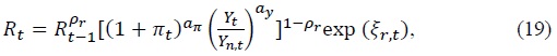
where  to a target value (
5. Aggregation
Aggregate consumption and aggregate hours are given by

and

Since there is no borrowing and lending between unconstrained households and HtM households in the closed economy TANK model, the net bond supply equals zero in equilibrium, i.e.
Aggregate dividend and bond holdings also satisfy


6. Equilibrium
Aggregating individual output across firms, one finds a wedge between the aggregate output

where 
Goods market clearing in home country requires that

and the output in the rest of the world which equals consumption in the rest of the world follows an AR(1) process.
(25) and (26) can be simplified as

The domestic and foreign bonds market clearing conditions are given by

while the equity market clearing condition implies that Θ
III. Quantitative Evaluations
In this section, we will address business cycles in Korea utilizing the specified small open economy TANK model along King and et al. (1988) and Woodford (2003).
1. Linearized Equilibrium Conditions
Assume that the fiscal authority implements an employment tax/ subsidy to attain the efficient steady state. Then, the log-linearized equilibrium conditions around the steady state can expressed in terms of 10 endogenous variables { as follows


and i.i.d. process
2. Estimation Methods
A subset of the model’s parameters is fixed in advance for the maximum likelihood estimation. The steady-state values of π and r are taken from the average inflation rate and nominal interest rate in the sample periods. The value of y is taken from the average level of detrended, per-capita GDP in the data. The elasticity of intertemporal substitution (σ⁻¹) and the Frisch labor supply elasticity (ν⁻¹) are set to 0.5 and 1, respectively, as in Galí (2008) and Woodford (2003). Next, the degree of goods market openness (θ) is set to 0.4 which corresponds to the average share of importables to GDP.
In the estimation, the dynamics of the system can be more compactly expressed in terms of six endogenous variables { by eliminating the consumption of each household as well as the terms of trade from the equilibrium conditions with the relevant definition. In this system, the state vector at period t,
  a monetary shock (
The model has 13 parameters,  Let the vector
  keep the track of state variables, and the vector
  track the flow variables whose values are the logarithmic deviations of detrended output, consumption, inflation rate, the real exchange rate, and the short-term nominal interest rates and net foreign asset holdings from their average. The equilibrium systems can be written as


where  are matrices of dimension 10×10,10×4,and 6×10 that depend on both unconstrained and constrained households’ tastes, firms’ pricing strategies, as well as the monetary authority’s policy rules. Here
  follows a normal distribution with zero mean and diagonal covariance matrix
  We apply the Kalman filter to form the log-likelihood function and estimate the values of unknown parameters using the observations.
IV. Empirical Results
The data taken from the Bank of Korea are quarterly and run from 1976:3Q through 2018:4Q. First, seasonally adjusted figures for real GDP is used to measure output. Quarterly changes in the seasonally adjusted GDP deflator and quarterly averages of the one-day call rate yield the measure of inflation and nominal interest rate. The US/Won nominal exchange rate is used to get the real exchange rate.
The Kalman filter can be used to construct the other parameter values, α, λ,
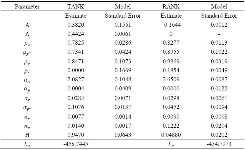
Table 1 presents maximum likelihood estimates of relevant parameters and the corresponding standard errors in the first subsample period running from 1976:3Q through 1997:2Q. The estimates for α and λ imply that firms have reoptimized their prices every six month on average, and about 27% of households are constrained households in the first subsample period. Under the null hypothesis that λ=0, the likelihood ratio statistic LR = 2(
Next, Table 2 displays the decomposition of forecast error variances in detrended output, inflation, the nominal interest rate, and the real exchange rate into components to each of the model's four orthogonal disturbances. The table shows that the domestic productivity shock has dominated in the variations of output at all horizons by accounting for more than 85 percent of unconditional variance of output, while the foreign productivity and monetary policy shocks have played a moderate role in output variations at short horizon. The monetary policy shock has been by far the dominant factor in the fluctuations of inflation at short and medium horizons by accounting for more than 40 percent of the unconditional variance of the inflation rate at the corresponding horizons. The domestic productivity and demand shocks have played an important role in the variations of inflation at all horizons by accounting for 20 percent of the unconditional variance of inflation rate at the corresponding horizons.
The demand shock has dominated in the behavior of the policy rate during a high economic growth era in Korea. The foreign productivity shock has dominated in the behavior of an international relative price by accounting for more than 75 percent of the unconditional variance of the international relative price at all horizons, while the contribution of the monetary policy shock to the variation of the real exchange rate is nil.
Table 3 presents maximum likelihood estimates of the deep parameters in the second subsample periods, i.e., after the Asian financial crisis, but before the Great Recession, 1998:1Q-2007:2Q. To restore the health of Korean economy hit by the Asian financial crisis, Korea government has implemented some restructuring polices to allow more flexibility in labor market as well as domestic and international financial markets. The market oriented economic policies have increased the share of nonregular or part-time workers and made the housing market as well as the credit market unstable. To deal with the increase in housing prices and credit booms, the government intervened in the housing market with macroprudential tools such as LTV and DTI for the first time to cool down the market. The government’s effort to cool down the housing market and the structural change in the labor market have substantially increased the fraction of households in the second subsample period. The large estimate of λ echoes the prevalence of the negative effect of the unprecedented Asian financial shock intertwined with government’s prudential policy on households.
The large estimate of
Table 4 displays the decomposition of forecast error variances in relevant variables into components attributable to each of the model’s orthogonal disturbances. The table shows that the domestic productivity has heavily contributed to output variations at all horizons, and the contribution of the monetary policy shock to output fluctuations is nil during the second subsample period. Table 4 also shows that the effect of the foreign country on the Korean economy has substantially increased as Korea has moved from a managed or pegged exchange rate regime to the flexible exchange rate regime with an inflation targeting rule after the Asian financial crisis. The foreign productivity shock has contributed heavily to the variations of inflation rate and interest rate by accounting for more than 30 percent of the unconditional variance of interest rate and the exchange rate at all horizons. In addition to the dominant role of a monetary policy shock, the preference shock has also contributed to the fluctuation of inflation during the second subsample periods. Since the monetary policy has been conducted to stabilize the price, the effect of a monetary shock on the key macroeconomic variables except inflation is nil as in Table 4.
Table 5 presents maximum likelihood estimates of the deep parameters during the Great Recession, 2007:3Q-2018:4Q. At first glance, the estimate for λ which is comparable to the one in the first sub-sample period might signal that Korea has successfully overcome the Asian financial crisis. But it might be the result of households’ precautionary behavior in the Great Recession. The higher uncertainty about what is going on can force households to cut consumption and save more. The small estimate of the nominal price rigidity α implies that the monetary policy can be ineffective in increasing output at the cost of inflation. Also notice that the monetary policy coefficient
Table 6 displays the decomposition of forecast error variances in relevant variables into components attributable to each of the model’s orthogonal disturbances. First, note that neither a monetary policy shock nor a preference shock is relevant to the variations in output. The domestic productivity shock has been the dominant factor in the variations of output by explaining about 80 percent of the unconditional variance of output at all horizons. The foreign productivity shock has substantially contributed to the fluctuations of output by explaining about 20 percent of output variations. As the monetary authority has tried to boost the aggregate demand by manipulating its policy rate, the effect of a monetary policy shock on the unconditional variance of inflation is larger in the third subsample periods than the ones in the first and second subsample periods at short and medium horizons. The foreign productivity shock has played an important role in the variations of inflation and interest rates, in addition to the fluctuation of the international relative price. Notice that the contrition of a monetary policy shock to the variations of other relevant variables is nil, implying that the monetary policy is ineffective to boost the economy with very low interest rate, i.e., near the zero-lower bound.
Figure 2 displays the impulse response function of some selected variables to a positive domestic productivity shock. The circle lines  the star lines
  and the dotted lines
  denote the response of relevant variables to the shock in the first, second, and the third subsample periods, respectively. The real exchange rate depreciates to the positive domestic productivity shock with the expansion of domestic output. The strong increase in output entails a fall of inflation rate to the shock in the first subsample period, which induces the monetary authority to cut its interest rate to stabilize the price as in Figure 1. However, a moderate expansion of output to the positive domestic productivity shock generates muted inflation, which induces the monetary authority to mildly adjust its policy rate in the second and third subsample periods. Notice that there is a very mild variation during the third sub-period, wherein the policy rate is near the zero-lower bound during the Great Recession period.2
Figure 3 presents the impulse response function of some selected variables to the foreign productivity shock in the first, second, and third subsample periods. The effect of foreign productivity shock on output is milder than the effect of domestic productivity shock, but its effect on the real exchange rate is much larger than the effect of the domestic productivity shock since the foreign output entails a proportional change in the international relative price through the risk-sharing condition. After the Asian financial crisis with the financial liberalization in Korea, the effect of foreign productivity shock on the Korean economy has been stronger than before the Asian financial crisis.
Figure 4 displays the impulse response function of some selected variables to the domestic preference productivity shock in the relevant subsample periods. The positive impact of domestic demand shock on output is expansionary during the first subsample period, while its effect on domestic economy activity is mild in the second and third sample sub-periods wherein the boosting effect of domestic demand shock has been limited with the financial liberalization in Korea.
Figure 5 shows the impulse response function of an interest rate shock to the selected variables. There are stronger responses of relevant variables to the shock in the first subsample period than in the second and third subsample periods. The muted response of output and inflation associated with a mild increase of the policy rate during the second and third subsample periods displays that the monetary authority has successfully conducted its policy to stabilize the economy with an adoption of the inflation targeting rule after the Asian financial crisis.
2)To get some intuition on the relevance of the TANK model over the business cycle in Korea, I have added impulse response functions of the RANK model in the appendix.
V. Concluding Remarks
This paper specifies a simple two-agent small open economy new Keynesian model with incomplete financial market, and then investigates the role of HtM households in the contribution of each shock to business cycles in Korea via maximum likelihood estimation since mid-1970s. The paper finds that there is a substantial fraction of constrained households which has played an important role over the business cycles in Korea and the estimated model reveals that the TANK model performs better than the RANK model in explaining business cycles in Korea.
The cost-push has played a pivotal role in the behavior of output over the business cycle, while the monetary policy shock has heavily contributed to the variation of inflation in the era of high economic growth. The monetary policy which was very loose to accommodate the high demand for liquidity during the first subperiod turned into proactive in controlling the inflation during the second subperiod as the Bank of Korea adopted the inflation targeting rule in 1998. Both the foreign productivity and cost push shocks have dominated over the business cycles in the third sub-period with the Great Recession, while the monetary policy shock has a limited effect on the economy near the zero-lower bound.
Tables & Figures
Figure 1.
Fluctuations of Key Macroeconomic Variables in Korea

Notes: All variables are detrended using quadratic methods to remove nonstaionary components. Output, inflation, interest rate, and real exchange rate are expressed in annual percentage times 100.
Table 1.
Maximum Likelihood Estimates and Standard Errors (1976:3Q-1997:2Q)

Note:
Table 2.
Forecast Error Variance Decompositions (1976:3Q-1997:2Q)

Table 3.
Maximum Likelihood Estimates and Standard Errors (1998:1Q-2007:2Q)
Note:
Table 4.
Forecast Error Variance Decompositions (1998:1Q-2007:2Q)
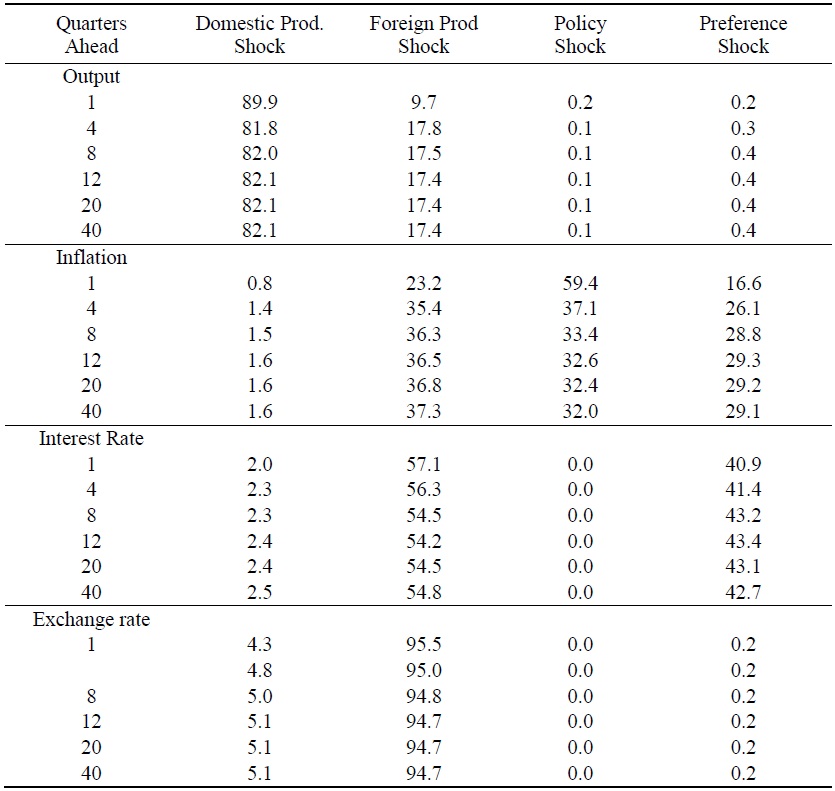
Table 5.
Maximum Likelihood Estimates and Standard Errors (2007:3Q-2018:4Q)

Note:
Table 6.
Forecast Error Variance Decompositions (2007:3Q-2018:4Q)

Figure 2.
Impulse Response Function to a Domestic Productivity Shock

Notes: The lines with circles, the lines with stars, and the dotted lines display the response of selected variables to a one-standard deviation of positive domestic productivity innovation in the first subperiods (1976:3Q-1997:2Q), the second sub-periods (1998:1Q-2007:2Q), and the third sub-periods (2007:3Q-2018:3Q).
Figure 3.
Impulse Response Function to a Foreign Productivity Shock

Notes: The lines with circles, the lines with stars, and the dotted lines display the response of selected variables to a one-standard deviation of positive foreign productivity innovation in the first subperiods (1976:3Q-1997:2Q), the second sub-periods (1998:1Q-2007:2Q), and the third sub-periods (2007:3Q-2018:3Q).
Figure 4.
Impulse Response Function to a Preference Shock

Notes: The lines with circles, the lines with stars, and the dotted lines display the response of selected variables to a one-standard deviation of positive domestic preference innovation in the first subperiods (1976:3Q-1997:2Q), the second sub-periods (1998:1Q-2007:2Q), and the third sub-periods (2007:3Q-2018:3Q).
Figure 5.
Impulse Response Function to an Interest Rate Shock

Notes: The lines with circles, the lines with stars, and the dotted lines display the response of selected variables to a one-standard deviation of negative domestic interest innovation in the first subperiods (1976:3Q-1997:2Q), the second sub-periods (1998:1Q-2007:2Q), and the third sub-periods (2007:3Q-2018:3Q).
APPENDIX: Steady State and Empirical Model for Estimation
A subset of the model’s parameters is calibrated in advance before applying the maximum likelihood procedure to estimate key parameters. The steady state values of the inflation rate and nominal interest rate are used to set
We assume the government implements a taxation or subsidization τ and redistributes the proceedings in a lump-sum fashion TR to attain an efficient steady state as in the literature (Bilbiie, 2008; Gali et al., 2007). Hence, there are zero profits at the steady state, since firms set marginal cost pricing and
Next, suppose that data are available on output

Then, the empirical model can be expressed as

where
and the vector of serially uncorrelated innovations  is assumed to be normally distributϵ with zero mean and diagonal covariance matrix
Let  and
and  Then,
Then,  Hence,
  with
with 
Then,  and
and 
The sequences of

And

given the initial values.
The innovations  can then be used to form the log likelihood function for
  as
as

Appendix Tables & Figures
Figure A1.
Impulse Response Function to a Domestic Productivity Shock: RANK Model

Figure A2.
Impulse Response Function to a Foreign Productivity Shock: RANK Model
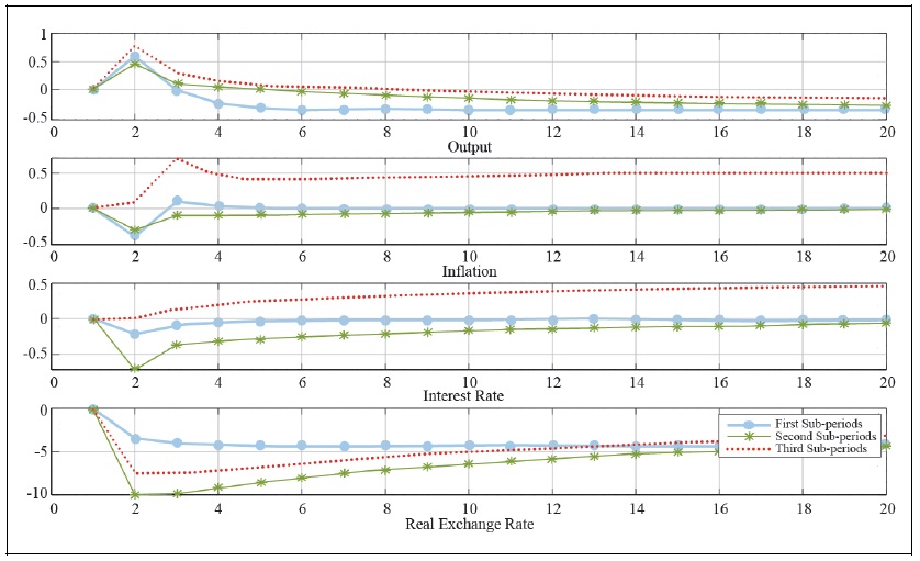
Figure A3.
Impulse Response Function to an Interest Rate Shock: RANK Model

References
-
Auclert, A. 2018. “Monetary Policy and the Redistribution Channel.”
Mimeo . -
Auclert, A., Rognlie, M. and L. Straub. 2019. “The Intertemporal Keynesian Cross.”
Mimeo . -
Benigno, P. 2009. “Price Stability with Imperfect Financial Integration.”
Journal of Money, Credit, and Banking , vol. 41, pp. 121-149.
-
Bilbiie, F. O. 2008. “Limited Asset Market Participation, Monetary Policy, and Inverted Aggregate Demand Logic.”
Journal of Economic Theory , vol. 140, pp. 162-196.
-
Bilbiie, F. O. 2019. “Monetary Policy and Heterogeneity: An Analytical Framework.”
Mimeo . -
Campbell, J. and G. N. Mankiw. 1989. “Consumption, Income, and Interest Rates: Reinterpreting the Time Series Evidence, in Blanchard, O and S. Fisher. (eds.)”
NBER Macroeconomics Annual , pp. 185-216. MIT Press. -
Dixit, A. and J. Stiglitz. 1977. “Monopolistic Competition and Optimum Product Diversity.”
American Economic Review , vol. 67, pp. 297-308. -
Debortoli, D. and J. Galí. 2019. “Monetary Policy with Heterogeneous Agents: Insights from TANK Modes.”
Mimeo . -
De Paoli, B. 2009. “Monetary Policy and Welfare in a Small Open Economy.”
Journal of International Economics , vol. 77, no. 1, pp. 11-22.
-
Galí, J. 2008.
Monetary Policy, Inflation and the Business Cycle , Princeton University Press. -
Galí, J., López-Saildo, D. and J. Vallés. 2007. “Understanding the Effects of Government Spending on Consumption.”
Journal of European Economic Association , vol. 5, no. 1, pp. 227-70.
-
Jung, Y. 2022. “Inspecting Business Cycles in Korea through the Lens of the TANK Model.”
Korean Economic Review , vol. 38, no. 1, pp. 109-139. -
Jung, Y. and Y. Kim. 2019. “Liquidity Constraint, Consumption Volatility and Consumption Gap.”
Kyung-Jae Bunseok Panel , vol. 25, no. 2, pp. 99-155. (in Korean) -
Kaplan, G., Moll, B. and G. L. Violante. 2018. “Monetary Policy According to HANK.”
American Economic Review , vol, 108, no. 4, pp. 697-743.
-
King, R. G., Plosser, C. and S. T. Rebelo. 1988. “Production, Growth and Business Cycles: I. The Basic Neoclassical Model.”
Journal of Monetary Economics , vol. 21, no. 2-3, pp. 195-232.
-
McKay, A., Nakamura, E. and J. Steinsson. 2016. “The Power of Forward Guidance Revisited.”
American Economic Review , vol. 106, no. 10, pp. 3133-3158.
-
Schmitt-Grohé, S. and M. Uribe. 2003. “Closing Small Open Economy Models.”
Journal of International Economics , vol. 61, pp. 163-185.
-
Woodford, M. 2003.
Interest and Prices: Foundations of a Theory of Monetary Policy , Princeton University Press. -
Yun, T. 1996. “Monetary Policy, Nominal Price Rigidity, and Business Cycles.”
Journal of Monetary Economics , vol. 37, pp. 345-370.