

- EAER>
- Journal Archive>
- Contents>
- articleView
Contents
Citation
| No | Title |
|---|---|
| 1 | Key Success Factors for Export Structure Optimization in East Asian Countries Through Global Value Chain (GVC) Reorganization / 2025 / Systems / vol.13, no.1, pp.22 / |
| 2 | Adjustment Cost on Investment and Under-Utilization of Maximum Installed Capacity in South Korean Business Cycle - A Bayesian New Keynensian Model / 2025 / ECONOMICS / vol.13, no.1, pp.1 / |
Article View
East Asian Economic Review Vol. 28, No. 3, 2024. pp. 277-314.
DOI https://dx.doi.org/10.11644/KIEP.EAER.2024.28.3.437
Number of citation : 2View
281
Download
204
Real Exchange Rate Misalignment and Economic Fundamentals in Korea
|
|
Sungkyunkwan University |
|---|

Abstract
This study analyzes the response of economic fundamentals to a misalignment shock of the real effective exchange rate in Korea. The estimation results of the equilibrium exchange rate determination model and time series model show that there is no significant difference in the direction of the deviation from equilibrium and that the won is significantly undervalued during the period before 1988, or during the currency and global financial crises. The cumulative impulse response analysis of the VAR model over the full period shows that an upward shock to the deviation from the equilibrium exchange rate reduces the GDP gap and inflation rate, while the effect on the call rate is not statistically significant. Furthermore, an upward misalignment shock initially worsens the goods and services balance, but the deficit in the goods and services balance shrinks significantly over time. In rolling regressions analysis, the entire sample is divided into two periods to estimate the impulse response function from the first period, and then the same procedure is repeated by moving the sample forward one by one. The cumulative impulse response results show that, as is the case for the full period, a positive exchange rate misalignment shock initially reduces the GDP gap, inflation, and worsens the goods and services balance, but the impact of this upward shock on these variables becomes increasingly weaker in the more recent sample. It also shows that the negative impact of upward shocks on the current account is smoothed out more recently during periods of undervaluation than during periods of overvaluation.
JEL Classification: C5, F3, F4
Keywords
Real Effective Exchange Rate Misalignment, VAR, Impulse Response, Rolling Regressions
I. Introduction
Korea is a small open economy, and as shown in the trade openness in Figure 1, the share of exports and imports in GDP has been exceeding 50% for most of the past half century, except for the first half of the 1990s, and has risen to over 100% in the early 2010s. This high share of exports and imports means that exports and imports, especially exports, have a very large impact on economic growth in an era of high economic growth, but also that exports are highly dependent on global economic conditions and can be significantly destabilized by foreign factors. Meanwhile, there are many factors that determine exports, but the most important factor that affects exports in the short term is the exchange rate.
During the 1986 Asian Games and the 1988 Seoul Olympics, Korea’s rapid economic growth was fueled by large current account surpluses, which had never been experienced before. However, the U.S. Treasury Department designated Korea as a currency manipulator in 1988, and in March 1990, Korea switched its exchange rate regime from a basket of currencies to a market average exchange rate, and the current account deficit returned. In this way, exchange rates can have a significant impact on economic growth by affecting imports and exports, but exchange rates can also be greatly affected by them. For example, after 1996, Korea experienced a currency crisis as the current account deficit widened due to the plunge in semiconductor prices and the economic recession deepened, and the exchange rate system was converted to a free-floating exchange rate system in December 1997. The massive outflow of foreign exchange led to a collapse in the value of the won, which led to an inflationary spiral, while the collapse in the value of the won subsequently revived price competitiveness, allowing for a large current account surplus and high economic growth. A similar situation occurred during the global financial crisis.
In the pre-crisis period, Korea's exports and imports were mainly centered on the United States and Japan, especially exports to the United States and imports from Japan, but since the 2000s, Korea has been trading more with China than with the United States and Japan. However, as Table 1 shows, exports to China have been declining in recent years, while exports to United States have been recovering, and exports to Southeast Asia, including Vietnam, have been steadily increasing. As trading partners become more diverse and the proportion of exports and imports by country or region changes significantly, the effective exchange rate is expected to have a greater impact on imports and exports and economic growth because the effective exchange rate that considers the proportion of trading partners rather than the won/dollar exchange rate can better evaluate the price competitiveness of imported and exported goods. Therefore, this study aims to examine the impact of the effective exchange rate of the won on macroeconomic variables.1
In this study, I first estimate the equilibrium exchange rate using the real effective exchange rate provided by the OECD and other basic economic variables that affect the equilibrium exchange rate, such as terms of trade, openness, productivity, government spending, and international interest rates. The long-term equilibrium exchange rate is estimated through time series models as well as existing theoretical models, and the deviations or gaps from the equilibrium exchange rate are extracted. Next, I examine how the misalignment from the equilibrium real effective exchange rate dynamically affect GDP, consumer price index, call rate, balance of goods and services, etc. The estimation model is a four- or five-variable VAR model with dummy variables for the period of the currency crisis and the global financial crisis. In addition, since the parameters may be time-varying or regime-switching during the entire period of analysis, I divide the entire period of analysis into two and use rolling regressions to examine how the response of macroeconomic variables to the real exchange rate shocks varies over time.
The results of estimating the equilibrium exchange rate using the theoretical and time series models indicate that there is no significant difference in the direction of the deviation from equilibrium and that the Korean won was significantly undervalued during the period before 1988 when Korea was designated as a currency manipulator, and during the currency crisis or the global financial crisis. The VAR model estimation results show that a positive exchange rate misalignment shock depresses the GDP gap and consumer prices, while slightly increasing the call rate, but not statistically significant. In addition, the goods and services balance initially deteriorates with a positive exchange rate misalignment shock, but recovers over time. In the case of the rolling regressions, the responses of the GDP gap, inflation, and the balance of goods and services to exchange rate misalignment shocks become smaller in the more recent sample. It also shows that the negative impact of upward shocks on the current account is smoothed out more recently during periods of undervaluation than during periods of overvaluation.
This paper is organized as follows. Section II first reviews the existing empirical studies on the real effective exchange rate at home and abroad, and then discusses the similarities and differences between this study and the existing studies. Section III estimates the equilibrium exchange rate determination models. In Section IV, I analyze the dynamic response of macroeconomic variables to deviations from the equilibrium exchange rate. Section V discusses the policy implications of the estimation results for our economy. Section VI summarizes our findings and draws conclusions.
1)
Ⅱ. Literature Review
As an extreme example, Figure 3 shows that the misalignment from the equilibrium real effective exchange rate of the won is positive in the period prior to the fourth quarter of 1997, when the currency crisis occurred. This implies that the real effective exchange rate is overvalued, and Korea experiences an excessive current account deficit and recession just before the Korean won depreciates due to the currency crisis.
Many empirical studies have suggested that such overvalued real exchange rates not only reduced economic growth by reducing exports, but also increased the likelihood of currency crises and political instability.2 Ghura and Grennes (1993), Rodrik (2008), Elbadawi, Kaltani, and Soto (2012) showed that economic growth was lower when the real exchange rate was overvalued. In addition, Sekkat and Varoudakis (2000) and Sekkat (2016) demonstrated that in the long run, an overvalued real exchange rate reduced export volumes and suppressed export diversification. In addition, overvaluation of the real exchange rate in the long run can lead to currency crises and political turmoil, as we experienced in 1997 (e.g., Holtemöller and Mallick, 2013; Ambaw and Sim, 2021).
Recent studies have examined the short-run effects of real exchange rate misalignments on current account imbalances, output gaps, and financial gaps. Using a sample of 22 advanced economies, Gnimassoun and Mignon (2015) found that overvaluation of the real effective exchange rate increased the size and persistence of current account imbalances. Gnimassoun and Mignon (2016) also showed that the three macroeconomic imbalances - real exchange rate misalignments, current account imbalances (external imbalances), and output gaps (internal imbalances) - were closely linked, and that overvaluation of the real exchange rate exacerbated current account deficits. Comunale (2021) used 27-country data to show that misalignment shocks to the real effective exchange rate had a negative impact on the EU’s financial and output gaps. Meanwhile, Lewis, Martin, and Bella (2007) and Staehr and Vemeulen (2016) used the real exchange rate gap as a measure of competitiveness and found that negative competitiveness shocks lowered GDP growth in the eurozone, but had little explanatory power for domestic demand and the current account. Ambaw et al. (2023) used data from 22 countries in Asia-Pacific region and a panel VAR model to show that in the short run, real effective exchange rate shocks had a negative impact on cyclical fluctuations in some countries.
Table 2 summarizes the recent literature using panel data. Ambaw et al. (2023), analyzing data for 22 countries including Korea, found that the overall impact of an upward shock to misalignment on the output gap was not clear and varied across countries. On the other hand, Gnimassoun and Mignon (2016) found that an upward shock to misalignment had a negative impact on the current account balance of 22 developed economies, while Staehr and Vermeulen (2016) showed that this effect was not the same for 11 Euro area countries. When analyzing such a large number of countries using Panel VARs, it is difficult to obtain consistent results for key economic variables such as the output gap and current account balance due to cross-country heterogeneity. As just one example, the macroeconomic impact of departures from equilibrium exchange rates is not the same for Europe as it is for Asia, as outliers such as the Asian currency crisis, the European currency and fiscal crises, and the global financial crisis do not have the same impact on each country. In light of these disparate conclusions of existing studies, as well as the fact that the Korean economy is a small open economy with a high degree of openness compared to other countries, this study analyzes how a misalignment shock to the won/dollar exchange rate dynamically affects the Korean macroeconomy, especially the current account.3
In this study, I consider various types of structural models and time series models simultaneously to estimate the real equilibrium exchange rate in a more advanced way than previous studies. In order to alleviate the problem of endogeneity in the long-run equilibrium model of the real effective exchange rate, not only the OLS method but also Stock and Watson’s (1993) dynamic OLS (DOLS) method is used, and the partial adjustment equation, a special case of the error correction equation, is estimated in the short-run dynamic equilibrium model. I also estimate the long-term exchange rate trend using time series estimation methods, such as the HP (Hodrick and Prescott, 1997) filter and the bandpass (Christiano and Fitzerald, 2003) filter, and compare them with the equilibrium exchange rate estimates from the theoretical model. Unlike previous studies in Korea, this study goes a step further to examine the dynamic impact of deviations from the equilibrium real exchange rate on major macroeconomic variables. Since outliers such as the currency crisis and the global financial crisis may distort the estimation results of linear VAR models, I estimate VAR models and impulse response functions with dummy variables for these periods. In addition, Korea has experienced major changes in its overall economic, financial, and industrial structure, including economic growth, trade, and capital mobility, due to the currency crisis and the global financial crisis over the past half century. Therefore, this study conducts a rolling regressions analysis to examine how the impact of exchange rate shocks on macroeconomic variables changes dynamically due to these changes in the overall economic environment. Finally, I examine whether the misalignment shock has an asymmetric effect by dividing the analysis period into periods when the won/dollar exchange rate was overvalued and undervalued.
2)The theoretical models for determining the equilibrium exchange rate on which empirical analyses are based include the behavioral equilibrium exchange rate (BEER) model, the natural real exchange rate (NATREX) model, and the fundamental equilibrium exchange rate (FEER) model
3)Domestic studies include
Ⅲ. Equilibrium Exchange Rate Estimation
1. Estimation Methods
The real exchange rate is the nominal exchange rate adjusted to reflect changes in purchasing power by converting the price levels of both countries into the same unit of currency, while the real effective exchange rate is the exchange rate that represents the overall relationship between the domestic currency and the currencies of all trading partners. The effective exchange rate is divided into the nominal effective exchange rate and the real effective exchange rate. The real effective exchange rate (REER) is an index calculated by geometrically averaging the real exchange rate between the domestic currency and the currencies of major trading partners, weighted by trade volume. It indicates the overall price competitiveness of domestic goods and is expressed as follows.

where
As previous studies have shown, the real effective exchange rate of the won is an unstable time series with a unit root, so the purchasing power parity theory does not hold in the long run. Therefore, it is difficult to derive the equilibrium exchange rate from itself, so theoretical models have emerged to explain the unstable nature of the exchange rate using underlying macroeconomic variables. These theoretical models include the behavioral equilibrium exchange rate (BEER) model by Clark and MacDonald (1998) and the fundamental equilibrium exchange rate (FEER) model by Williamson (1994). The BEER approach measures the equilibrium exchange rate level in the medium and long run as the real exchange rate adjusts to the long-run equilibrium exchange rate through an econometric technique that establishes behavioral linkages between the real exchange rate and relevant economic variables. The FEER approach measures the real exchange rate that would equalize the current account and sustainable net capital flows at full employment. As such, the equilibrium exchange rate is generally defined as the real exchange rate at which both domestic and foreign equilibrium are achieved simultaneously (Edwards, 1989). Here, domestic equilibrium implies that the non-tradable goods market is in a sustainable equilibrium, while foreign equilibrium indicates that the current account deficit is financed by sustainable capital inflows. In general, to estimate the equilibrium real effective exchange rate that satisfies both internal and external balances, existing studies use terms of trade, net foreign assets, and foreign interest rate as external variables, and productivity, government expenditure to GDP, and trade openness as domestic variables.
In this study, I first regress the logarithmic real effective exchange rate on domestic and foreign underlying macroeconomic variables as follows.
where
I first estimate the case without the partial adjustment term and dummy variables in equation (2) by OLS and then compare it to the case with these terms. I also estimate the long-run equilibrium equation without lags and partial adjustment term in equation (2) by using the DOLS estimation method of Stock and Watson (1993), considering the four leading and lagging lags of the difference variables. As noted by Ball (2012), the partial adjustment model is a model that imposes certain constraints on the error correction model. As is generally recognized, the long-run equilibrium model is good at explaining long-term trends, while the error correction model is good at explaining short-term fluctuations. Therefore, in this study, I estimate the equilibrium real effective exchange rate without as well as with the partial adjustment term, and then substitute the estimated parameter values and the long-run trend values obtained using the HP filter for each domestic and external macroeconomic variable into equation (2) to obtain the equilibrium real effective exchange rate.
2. Estimation Results
The real effective exchange rate (
Figure 1 shows the evolution of the real effective exchange rate and the explanatory variables used to estimate the equilibrium exchange rate model. The real effective exchange rate has been declining significantly during the period before 1988, when the current account surplus exceeded $10 billion, during the currency crisis, and during the global financial crisis. Government expenditure as a share of GDP (
Before estimating the equilibrium exchange rate model, the ADF test for each level variable illustrates that
The estimation results in Table 5 show that regardless of the estimation equation, the parameters of the underlying economic variables have positive values, while the parameters of the dummy variables have negative values. First, the estimation results in (2-1) show that a 1%p increase in the share of government spending in GDP (
In (2-2), dummy variables
Figure 2 shows the logarithmic real effective exchange rate and the logarithmic equilibrium real effective exchange rate estimated from equation (2-1).8 They are shown as solid and dotted lines, respectively. Figure 3 displays the misalignment of the logarithmic real effective exchange rate from the logarithmic equilibrium real effective exchange rate.9
4)When the nominal exchange rate (
5)The money market rate is similar to the Bank of Korea’s call rate and is the same as the uncollateralized call rate (all transactions) from the first quarter 1997 to the fourth quarter of 2022.
6)Using
7)There is no significant difference in the estimates when the explanatory variables
8)The reason why net foreign assets (NFA) is not used in this study is that the period analyzed in this study is from the third quarter of 1976 to the fourth quarter of 2022, while net international investment position (NIIP) and net external assets (NEA) data provided by the Bank of Korea are available from the fourth quarter of 1994, and NFA data provided by the IMF is available from the fourth quarter of 2001. On the other hand, Ambar et al (2023) did not mention which data were used as Korea’s NFA data and how long it was used. Table A2 in the ONLINE APPENDIX of Ambar et al. (2023) showed that the explanatory power of NFA was low (see Appendix 1).
9)Please refer to Appendix 2 for more specific details.
Ⅳ. How to Estimate VAR and Rolling Regressions
1. Impulse Response Analysis
In this section, I use VAR models to examine the dynamic impact of deviations from the equilibrium real exchange rate on the domestic macroeconomy. The four- and five-variable VAR models used over the entire period of analysis are as follows.

where Δ
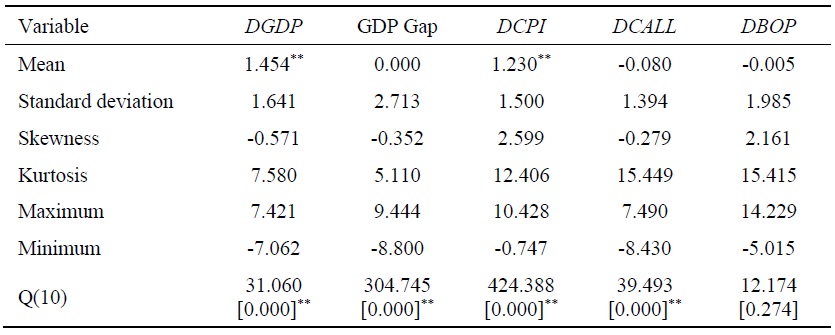
Before analyzing the impulse responses, I examine the behavior of the variables used in the analysis through Table 6 and Figure 4. In Table 6, the average GDP growth rate (
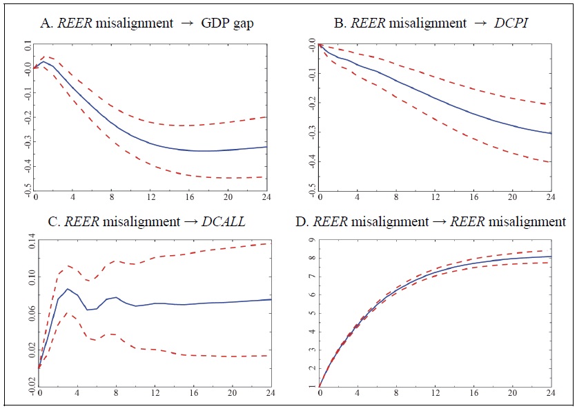
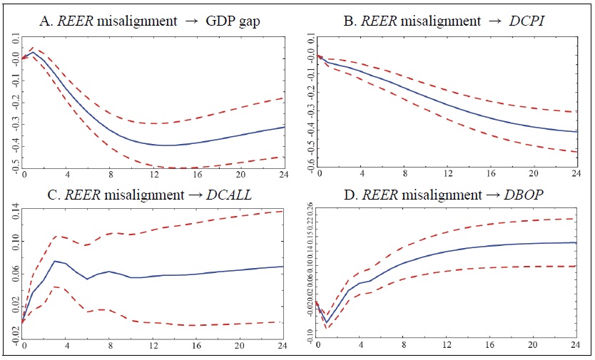
In this section, I first estimate a four-variable VAR model consisting of the GDP gap, consumer price inflation, the change in the call rate, and the real effective exchange rate misalignment. The real effective exchange rate misalignment is obtained through the simplest estimation equation (2-1) in Table 5. I estimate the impulse response function using the Cholesky decomposition, which is commonly used in existing studies because of its ease of estimation. In the case of Cholesky decomposition, the order of the variables is important, and unlike Ambaw. et al. (2023), who put the inflation rate in front of the GDP gap, I order the variables in the order of the GDP gap, inflation rate, interest rate change rate, and real effective exchange rate misalignment in the way that existing studies do. The number of lags of the VARs is set to 3 based on the AIC and AICc criteria.13
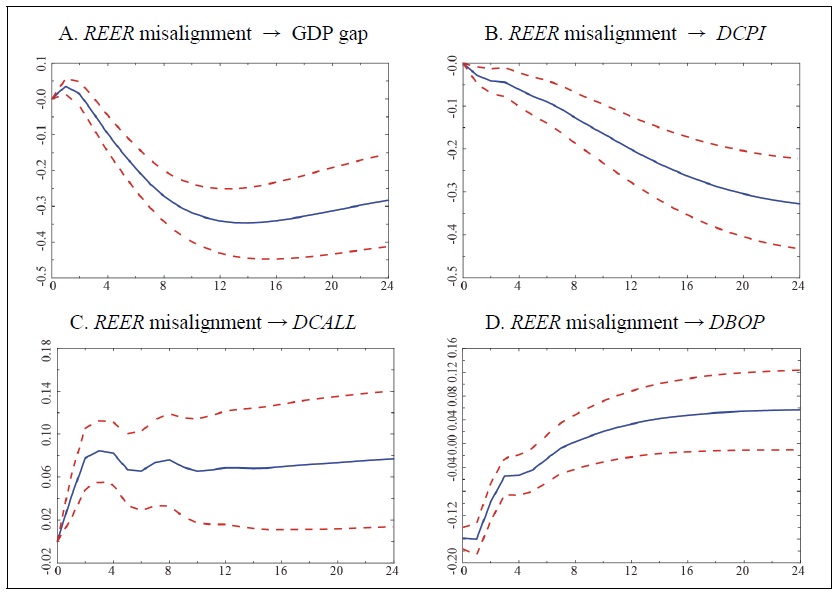
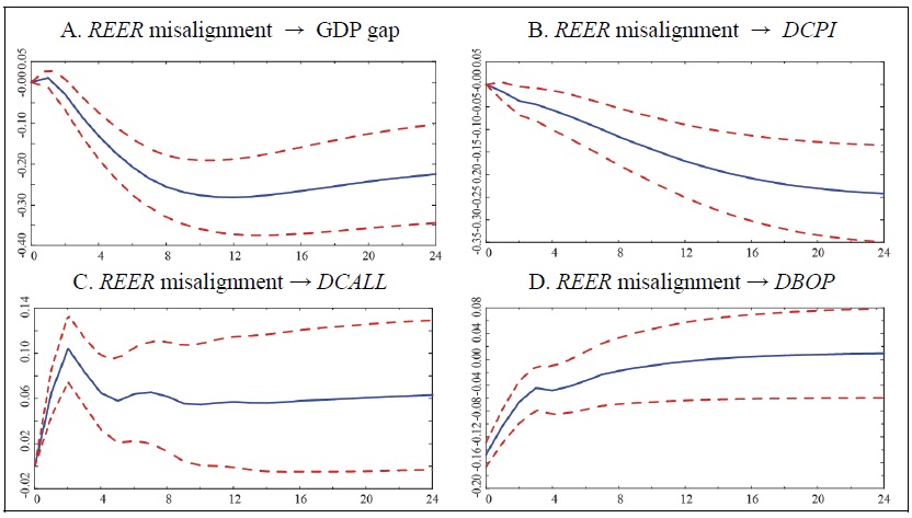
Figure 5 shows the cumulative response of each variable to a positive misalignment shock of real effective exchange rate. First, for a 1%p increase in the exchange rate misalignment, the GDP gap decreases by 0.337%p until the 18th quarter and then decreases slightly thereafter.14 In addition, when the exchange rate misalignment increases by 1%p, consumer price inflation continues to decline, falling by more than 0.3%p after 24 quarters. Meanwhile, the call rate increases by more than 0.07%p in the long run for a 1%p increase in the exchange rate misalignment. In Figure 5, the dotted lines above and below the solid line show the 90% confidence interval obtained by 1,000 iterations of bootstrapping using the actual distribution of the error term. In the case of the call rate, not only is the response small, but the confidence interval is very wide, indicating a lack of statistical significance.
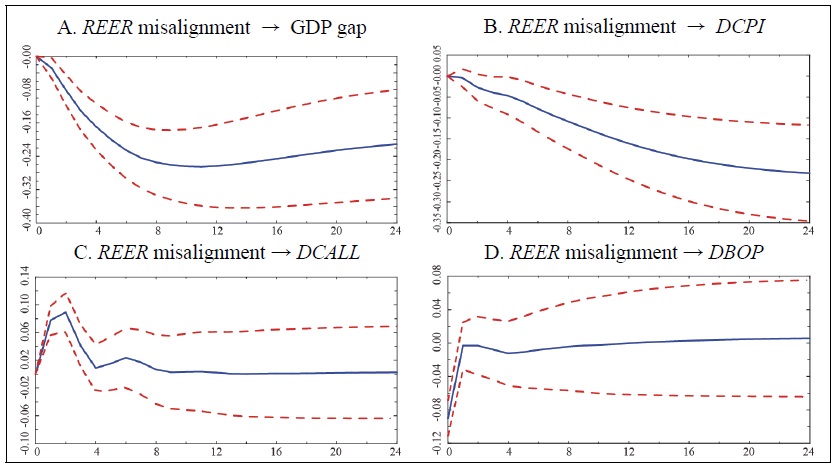
Recent studies have examined the impact of deviations from the equilibrium real effective exchange rate in the short run on current account imbalances as well as on growth and inflation. For example, Gnimassoun and Mignon (2015) and Gnimassoun and Mignon (2016) showed that an overvaluation of the real effective exchange rate worsened the current account deficit. Therefore, this paper examines the impact of the real exchange rate misalignment on the balance of payments using a five-variable VAR model that adds a variable for the balance of goods and services in addition to the four variables in Figure 5. The order of the variables is the GDP gap, inflation, interest rate change, real effective exchange rate misalignment, and change in the balance of goods and services. Change in the balance of goods and services is placed after the real effective exchange rate misalignment because of the contemporaneous causality between the two variables. The number of lags of the VARs is set to 3 according to the AIC and AICc criteria. In Figure 6, when the exchange rate misalignment rises by 1%p, the responses of the GDP gap, consumer price inflation, and call rate change are similar to the four-variable case. In the case of the balance of goods and services, the deficit of the balance of goods and services immediately increases by 0.158%p when the exchange rate misalignment increases by 1%p, but the deficit growth rate declines continuously thereafter, showing that the balance of goods and services turns into a surplus in the long run.15
2. Rolling Regressions Analysis
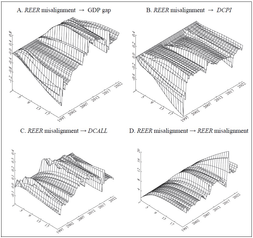
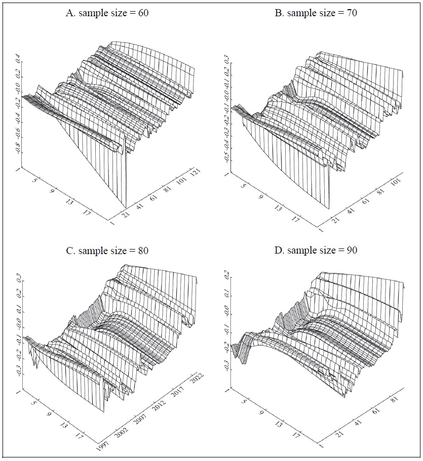
Figures 5 and 6 show the impact of a deviation shock from the equilibrium real exchange rate on macroeconomic variables using data from 1976 to 2022. However, since there were several crises during this nearly 50-year period, as well as regime switches from high growth and high interest rates to low growth and low interest rates, it is necessary to analyze the period in more detail as well as use dummy variables. For the rolling regressions analysis, I first estimate the cumulative response for the former sample of 80 quarters using the same estimation methodology used in Figures 5 and 6, and display it on the first y-axis in Figure 7. Next, the estimation sample is shifted one quarter while keeping the sample fixed at 80 quarters, and the cumulative response is obtained using data from the first quarter of 1977 to the fourth quarter of 1996 and plotted on the second y-axis. The same method is repeated, and finally, at the 106th time, the results are plotted on the y-axis for the last time, using the data from the first quarter of 2003 to the fourth quarter of 2022. When using the rolling regressions estimation method, the number of lags in the VAR model is determined each time using the AICc, and if the estimation period includes either or both the currency crisis and the global financial crisis, dummy variables for these are included in the estimate.16
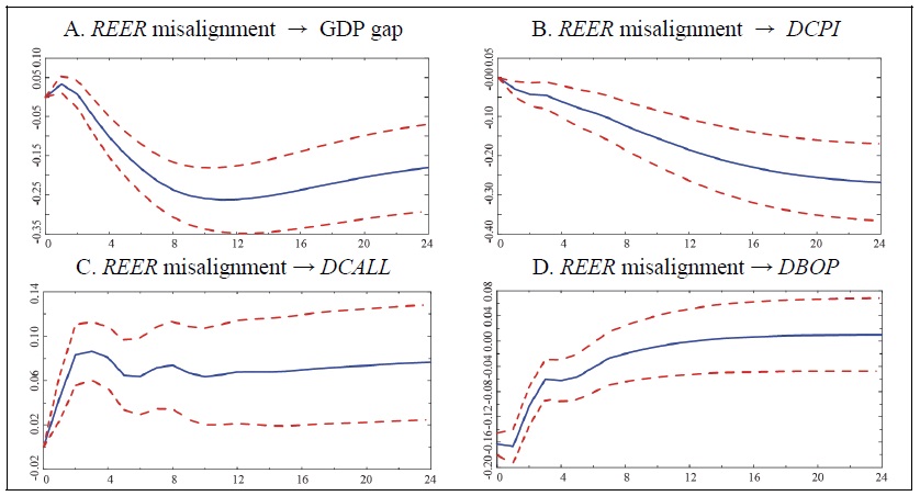
First, Figure 7.A displays the impact on the GDP gap of a 1%p upward misalignment shock of real exchange rate. For the entire period analyzed, the GDP gap cumulatively declines until the 18th quarter, and then the decline decelerates (see Figure 5.A). On the other hand, the rolling regressions estimation results show that the response of the
Figure 8 shows the five-variable case, which includes the goods and services balance. The impact of a 1%p upward misalignment shock of real exchange rate on the GDP gap, inflation, and the call rate change is not significantly different from the four-variable case in Figure 7. On the other hand, a positive 1%p misalignment shock of the real exchange rate leads to a large initial increase in the goods and services deficit over the full period and converges to zero in the long run (see Figure 6.D). But Figure 8.D shows that the goods and services deficit shrinks as more recent samples are used. In other words, when data from the 1980s and 1990s are used, the goods and services balance deficit appears large, but as data from the 2000s are included in the analysis period, the goods and services balance deficit is significantly reduced.
This study shows only the results when the sample estimation period used in the rolling regressions analysis is fixed at 20 years (80 quarters). However, the conclusion that the impact of an exchange rate misalignment shock on the GDP gap, inflation, and the balance of goods and services diminishes gradually in the more recent sample periods remains unchanged even when the sampling period is changed to 60, 70, 80, and 90 quarters, etc.17
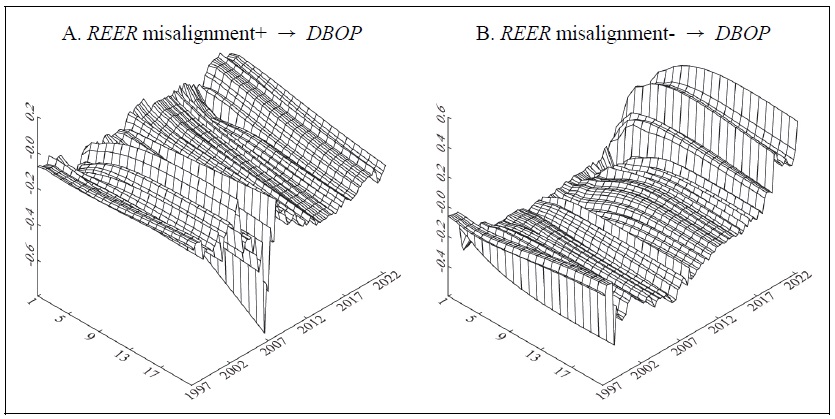
In order to check asymmetric effects, this study further distinguishes between overvaluation and undervaluation periods and examine how an upward misalignment shock in each period affects the current account. Figure 9 shows the impact of misalignment+ and misalignment- upward shocks on the current account using rolling regressions in a six-variable VAR model consisting of GDP gap, inflation, change in call rate, REER misalignment+, REER misalignment-, and change in goods and services balance. In Figure 9, misalignment+ (-) is a variable that takes on the value of the upward (downward) shock during periods when the REER misalignment is rising (falling) but is zero during periods when the REER misalignment is falling (rising). It shows that the negative impact of upward shocks on the current account is smoothed out more recently during periods of undervaluation than during periods of overvaluation. The results are the same when the order of misalignment+ and misalignment- is reversed.
In this way, the recent decline in the impact of the real exchange rate on the current account is due to an increase in the share of exports from technologically competitive industries such as automobiles, displays, and semiconductors rather than from industries with price competitiveness. In addition, the impact of the exchange rate on exports of intermediate goods rather than final goods has been weakening due to the sophistication of the export industry structure and the transition of major exporters to a global production system, which has dampened the impact of exchange rate fluctuations through overseas production, intra-firm trade, and the mitigation of exchange rate pass-through effects. Further research needs to be conducted on industry-specific effects in the future (see Lee and Kang, 2022).
10)As shown in
11)These dummy variables have been validated and used in many domestic and international papers. The won/dollar exchange rate started to rise in the Hong Kong and Singapore NDF markets around October 1997, and the IMF bailout was decided on November 21, 1997. The won/dollar exchange rate, which had fluctuated rapidly, began to stabilize after the first quarter of 1999. The KOSPI plummeted from the fourth quarter of 1997 and started to recover from the fourth quarter of 1998. Including the third quarter of 1997 or excluding the fourth quarter of 1998 does not make much difference to the estimation results, but I report the case of relatively high statistical significance. With the bankruptcy of Lehman Brothers on September 15, 2008, the U.S. subprime crisis spread into a global financial crisis, and in Korea, the won/dollar exchange rate soared and stock prices began to plummet in October. The global financial crisis soon transitioned into a global real crisis.
12)The ADF unit root test with 4 lags shows that the test statistics for the level variable and the difference variable of the call rate are -2.599 and -7.0156, respectively. I use the difference variable because the level variable has a unit root. The response of the current account to the misalignment shock is not significantly different when using level variables. There is also no significant difference in the main results when the interest rate difference between Korea and the United States (call rate-federal funds rate) is used instead of the call rate change.
13)Reversing the order of the variables does not make much difference to the conclusions (see Appendix 3). Since
14)When using a smoothing parameter of 1,600 instead of 16,000, the GDP gap also falls in response to an increase in the misalignment, but by a smaller amount. Using GDP growth and GDP per capita growth instead of the GDP gap, the growth rate also falls.
15)Please see the Appendix 4 for the impulse response results when using the real effective exchange rate misalignments obtained from estimation equations with dummy variables or constant terms. There is no significant difference in the responses to the different estimation equations, but the initial deficit in the goods and services balance converges to zero rather than a surplus in the long run when dummy variables are used.
16)When estimating the TVP-VAR model using these data, various variations in the size of the prior distribution and the number of variables or lags are tried, but in most cases, estimation is not possible, and even when estimation is possible, the results are unstable. On the other hand, when rolling regressions are used, stable estimation results are shown regardless of the sample size, lags, variables, etc.
17)Please see the Appendix 5.
Ⅴ. Policy Implications
In November 2023, the U.S. Department of the Treasury released its semiannual Report to Congress, which showed that Korea was removed from the U.S. exchange rate monitoring list for the first time in seven years since April 2016. Under the Trade Promotion Act of 2015, the U.S. designates a country as an in-depth analysis or watch list if it meets the following criteria: (1) a trade surplus with the U.S. of more than $15 billion in goods and services, (2) a current account surplus exceeding 3% of GDP, and (3) net purchases of U.S. dollars exceeding 2% of GDP for eight out of 12 months. Except for the first half of 2019, when only one criterion was met, Korea met two criteria. However, this time, as it met only one or less criteria for the second time in a row, it was excluded from the list of countries subject to observation. In addition to the Trade Promotion Act, the U.S. Treasury categorizes U.S. trading partners as currency manipulators and non-currency manipulators based on the Comprehensive Trade Act. Korea was designated as a currency manipulator in 1988 but was released two years later.
The empirical results of this study contribute to understanding the circumstances under which the U.S. designated Korea as a currency manipulator or a country subject to exchange rate observation from the perspective of international economics. The empirical results show that in the 1980s and 1990s, when the share of U.S. trade in total trade was large, there was an incentive to depreciate the won through adjustment of the real effective exchange rate or intervention in the foreign exchange market under the multicurrency basket system or the market average exchange rate system, respectively, because the undervaluation of the real effective exchange rate had a positive impact on economic growth and the business cycle as well as the current account despite inflation. As a representative example, the value of the won was significantly underestimated in the period immediately preceding 1988, when a current account surplus of $12.8 billion was recorded. However, empirical analysis demonstrates that as the positive impact of the undervaluation of the real effective exchange rate on the economy and the current account diminishes over time, the authorities have less incentive to intervene in the foreign exchange market because it is difficult to measure the benefits and costs of intervention. In other words, as Korea moves to a net external creditor country or a net external asset country due to the continuous surplus in the current account after the currency crisis, foreign direct investment and portfolio investment are activated, and the expansion of foreign investment not only replaces exports and jobs, but also plays a role in suppressing the appreciation of the won and the growth of imports through foreign currency outflows. In particular, the impact of the exchange rate on exports of automobiles, displays, and semiconductors has been reduced due to the sophistication of the export industry structure and the offshoring of production facilities. Therefore, it is more difficult than in the past to accurately measure the impact of the real effective exchange rate on macroeconomic variables when the proportion of trade with a trading partner changes significantly.
To summarize, a positive exchange rate misalignment shock lowers the GDP gap, inflation, and worsens the goods and services balance over the entire period, but the impact of this upward shock on these variables becomes increasingly weaker in the more recent sample. In particular, the negative impact of upward shocks on the current account is smoothed out more recently during periods of undervaluation than during periods of overvaluation. Therefore, although the costs and benefits of exchange rate shocks may vary significantly among different interest groups, it is not clear from the perspective of the national economy as a whole, so it is not advisable for policy makers to intervene in this area prematurely.
Ⅵ. Summary and Conclusions
This study uses real effective exchange rate data from 1976 to 2022 to dynamically analyze the impact of misalignments from the equilibrium real effective exchange rate on macroeconomic variables such as output gap, inflation, call rate, and balance of goods and services.
I estimate the real effective exchange rate misalignments using a theoretical model of equilibrium exchange rate determination and HP or bandpass filters. The explanatory variables used to estimate the equilibrium exchange rate in the theoretical model include government spending, openness, terms of trade, productivity, and U.S. interest rates. The estimation results show that there is no significant difference in the direction of the deviations for the long-run equilibrium exchange rate estimates based on the theoretical and time-series models, regardless of whether dummy variables or partial adjustment terms are included. The misalignments also show that the Korean won was significantly undervalued before the designation of the exchange rate manipulator in 1988 and during the currency crisis or global crisis.
The results of the cumulative impulse response analysis over the full period using a four- or five-variable VAR model show that a positive misalignment shock of the real effective exchange rate reduces the GDP gap and consumer price inflation, while it increases the change in the call rate, but the effect on the call rate is not statistically significant. In addition, a positive exchange rate misalignment shock initially worsens the goods and services balance, but over time, the goods and services balance deficit shrinks significantly.
Finally, since there are economic crises and regime switches during the entire analysis period of nearly half a century, I examine the impact of a positive exchange rate misalignment shock on macroeconomic variables through rolling regressions analysis. In rolling regressions analysis, the entire sample is divided into two groups to estimate the impulse response function from the first group, and then the same procedure is repeated by moving the sample forward one by one. The cumulative impulse response results show that, as is the case for the full period, a positive misalignment shock to the exchange rate initially reduces the GDP gap, inflation, and worsens the goods and services balance, but the impact of this upward shock on these variables becomes increasingly weaker in the more recent sample.
In summary, from a macroeconomic perspective, it is becoming increasingly more difficult than in the past to measure the benefits and costs of an unexpected misalignment shock from the equilibrium real effective exchange rate to the national economy.
Tables & Figures
Figure 1.
Movement of Macroeconomic Variable I
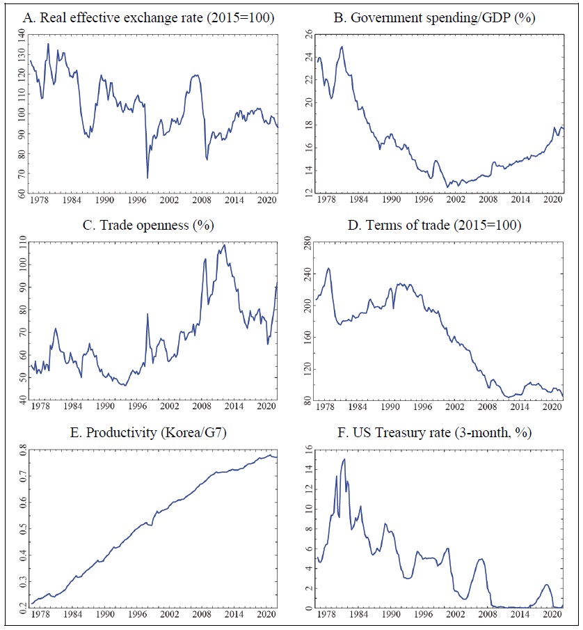
Note: Trade openness and terms of trade (TOT) refer to EXIP/GDP and net barter terms of trade index, respectively, and productivity (PROD) is estimated as the ratio of Korea/G7 after converting OECD’s annual data of GDP per person employed (US$, constant price) to quarterly data for Korea and G7.
Table 1.
Share of Exports and Imports by Region
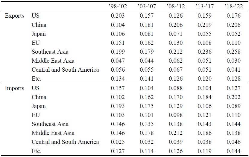
Source: Bank of Korea (5-year average)
Table 2.
Recent Literature for Panel Data Analysis
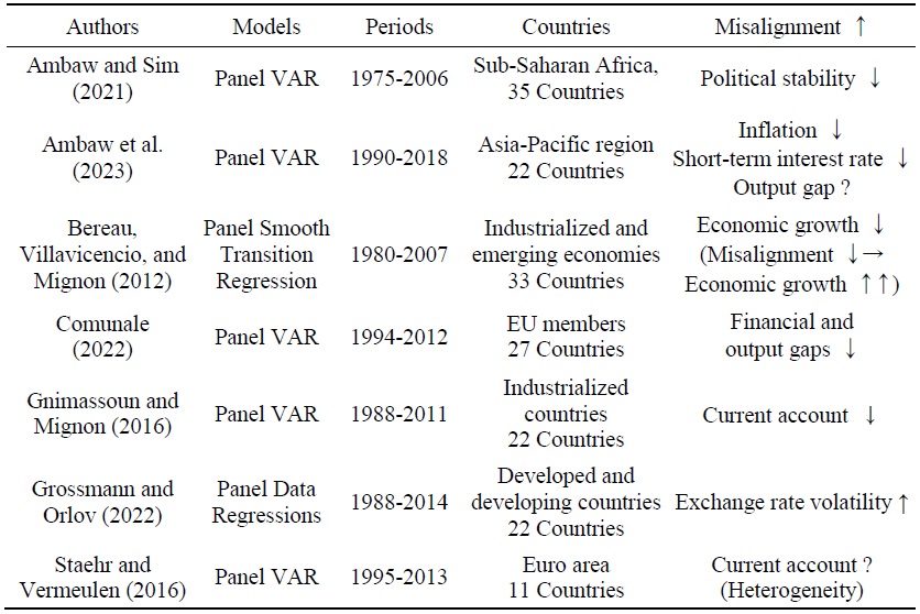
Table 3.
ADF Unit Root Test (lag=4)
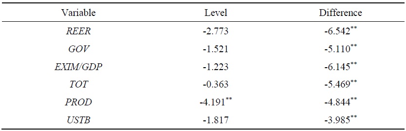
Notes: 1)
2) ** indicates significant at the 1% level.
Table 4.
Test of Cointegration: Johansen Test (lag=4)
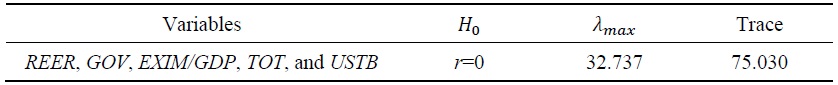
Notes: 1)
2) The 10% thresholds for
Table 5.
Equilibrium Exchange Rate Model Estimation Results
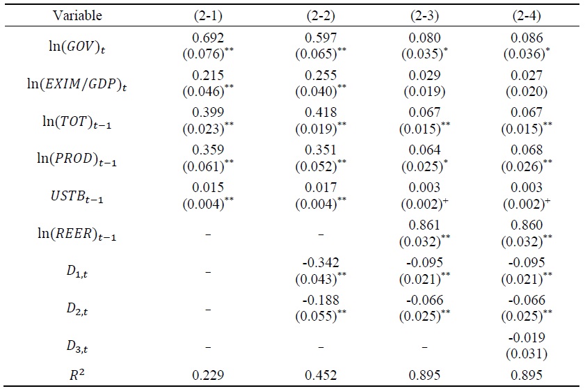
Notes: 1)
2) +, *, ** denote significance at the 10%, 5%, and 1% levels, respectively.
Figure 2.
Real Effective Exchange Rate and Equilibrium Real Effective Exchange Rate
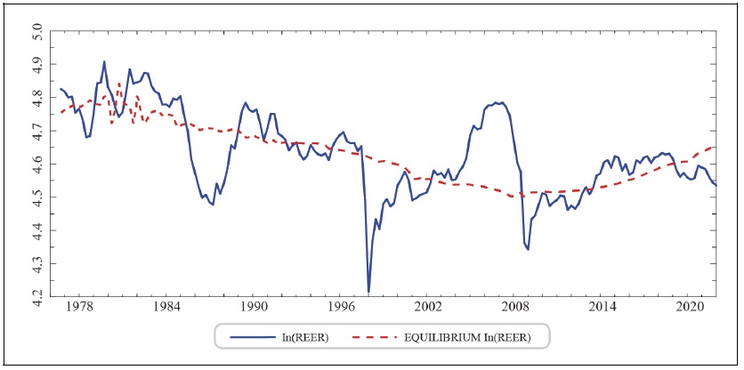
Figure 3.
Real Effective Exchange Rate Misalignment
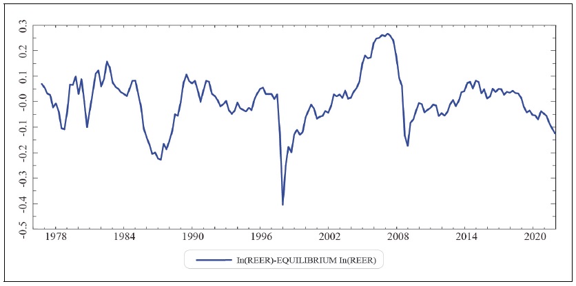
Table 6.
Basic Statistics
Notes: 1)
2) ** indicates significant at the 1% level.
3) Q(10) displays the Ljung-Box test statistic for 10th order serial correlation.
4) Values in [ ] indicate p-values.
Figure 4.
Movement of Macroeconomic Variable Ⅱ
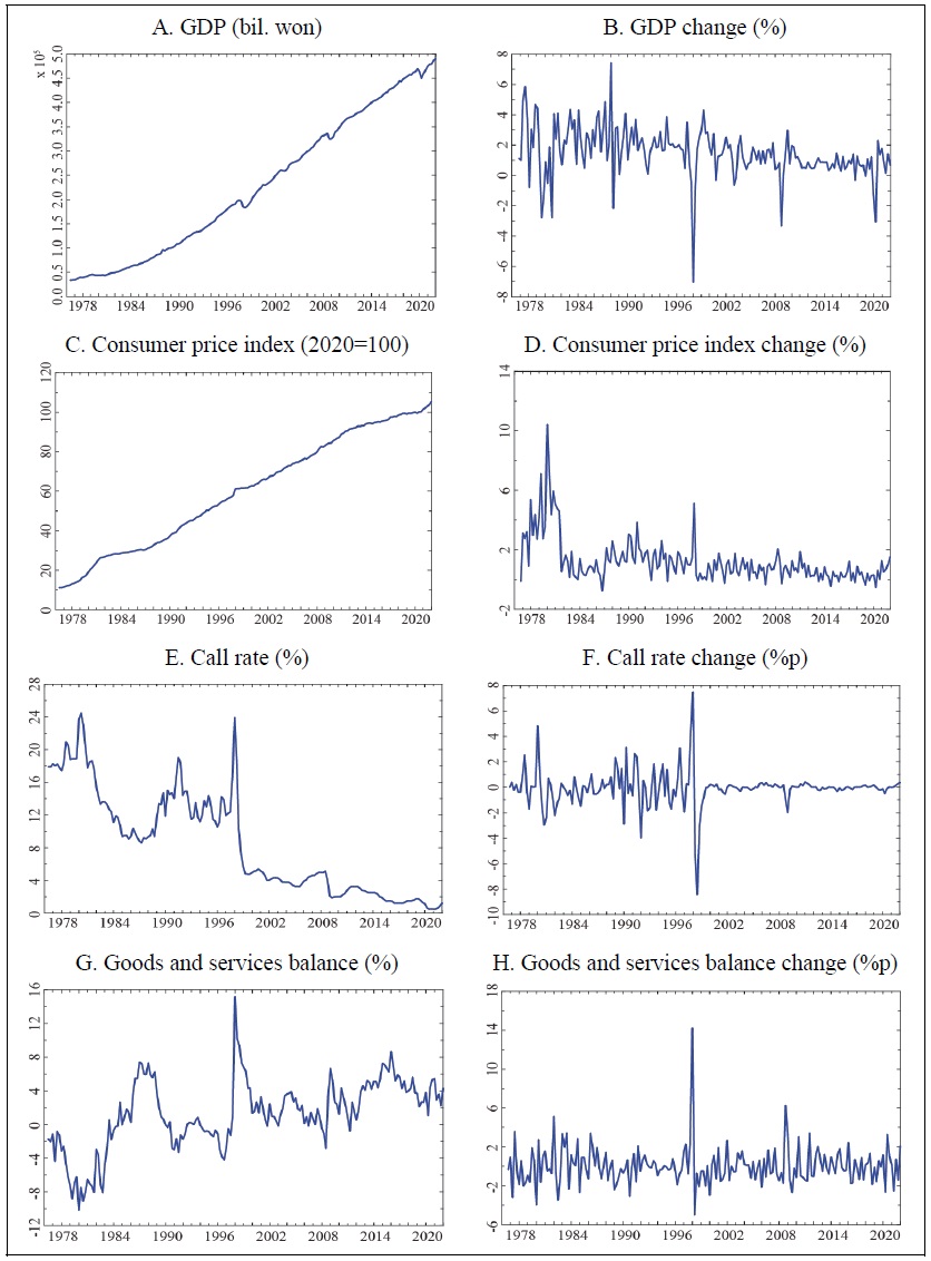
Figure 5.
Cumulative Response Curve (4 variables, lag: 3)
Note: 1)
Figure 6.
Cumulative Response Curve (5 variables, lag: 3)
Note:
Figure 7.
Cumulative Response Curve (4 variables, rolling regressions estimation)
Notes: 1)
2) After dividing the analysis period into 1976:Q4-1996:Q3 (80 quarters) and 1996:Q4- 2022:Q4 (105 quarters), I first estimate the cumulative response for the former sample of 80 quarters and display it on the first y-axis. Next, the estimation sample is shifted one quarter while keeping the sample fixed at 80 quarters, and the cumulative response is obtained using data from 1977:Q1 to 1996:Q4 and plotted on the second y-axis. The same method is repeated, and finally, at the 106th time, the results are plotted on the y-axis for the last time, using the data from 2003:Q1 to 2022:Q4.
Figure 8.
Cumulative Response Curve (5 variables, rolling regressions estimation)
Notes: 1)
2) After dividing the analysis period into 1976:Q4-1996:Q3 (80 quarters) and 1996:Q4- 2022:Q4 (105 quarters), I first estimate the cumulative response for the former sample of 80 quarters and display it on the first y-axis. Next, the estimation sample is shifted one quarter while keeping the sample fixed at 80 quarters, and the cumulative response is obtained using data from 1977:Q1 to 1996:Q4 and plotted on the second y-axis. The same method is repeated, and finally, at the 106th time, the results are plotted on the y-axis for the last time, using the data from 2003:Q1 to 2022:Q4.
Figure 9.
Cumulative Response Curve (6 variables, rolling regressions estimation)
Notes: 1)
2) misalignment+ (-) is a variable that takes on the value of the upward (downward) shock during periods when the REER misalignment is rising (falling) but is zero during periods when the REER misalignment is falling (rising).
3) The order of variables is GDP gap,
APPENDIX 1
Data on Reserve Assets, one of the Balance of Payments items provided by the Bank of Korea, is available from the first quarter of 1980. Therefore, I arbitrarily assume that Reserve Assets are zero from the third quarter of 1976 to the fourth quarter of 1979, and then estimate equation (2), which adds the share of Reserve Assets in dollar-denominated nominal GDP (seasonally adjusted nominal GDP divided by the average won/dollar exchange rate) (
APPENDIX 2
Figure A2 shows the deviation of the logarithmic real effective exchange rate from the logarithmic equilibrium real effective exchange rate. Since there are differences in standard deviations depending on the estimation method, I standardize the misalignments using the mean and standard deviation for ease of comparison. First, Figure A2.A displays the misalignments from Equation (2-1) and the case where the constant term is included in Equation (2-1). They are shown as solid and dotted lines, respectively, and are not significantly different, but the standard deviation is smaller with the constant term (9.342) than without (10.351). Figure A2 illustrates that the value of the won falls significantly just before 1988, when the current account surplus reached $12.8 billion and Korea was designated as a currency manipulator by the U.S. Treasury. After switching to the market average exchange rate system in March 1990, the misalignment was close to zero, and then, due to the semiconductor boom in 1995, the won became overvalued until just before the currency crisis. However, after the 1997 currency crisis, the won plummeted and recovered, but fell again in 2002 due to the credit card crisis, and then rose until just before the subprime crisis in the United States due to the large influx of foreign capital into the domestic stock market. As the subprime crisis turned into a global financial crisis, the value of the won plummeted again, but then rose relatively slowly due to the aftermath of the European fiscal crisis and the Lee Myung-bak government’s aggressive exchange rate policy to curb the rapid appreciation of the Korean won.
The reason why the won depreciated less after the global financial crisis than after the currency crisis is because the main cause of the currency crisis was domestic problems, while the global financial crisis was not caused by domestic problems but by the subprime crisis in the United States. The Korean won was relatively overvalued during the Park Geun-hye and Moon Jae-in administrations, but it has become undervalued again after the coronavirus outbreak.
Figure A2.B shows the misalignments from equations (2-1) and (2-3), where equation (2-3) includes the partial adjustment term and two dummy variables representing the currency crisis and the global financial crisis. There is a difference in the magnitude of the misalignments but little difference in the direction. According to Ball (2012), the partial adjustment model is a constrained error correction model, and the fact that the estimates of the long-run and partial adjustment models are not significantly different demonstrates that the long-run equation explains short-term fluctuations as well as long-term trends. Figure A2.C shows the misalignments estimated by the equilibrium model in (2-1) and the misalignments estimated by DOLS including the four leading and lagging lags of the difference variables in (2-1). There is no significant difference in the direction of the deviation change, but there is a relatively large difference in the magnitude of the change over time, with the standard deviation of the DOLS estimate being slightly larger at 11.331. Figure A2.D shows the misalignments from (2-1) and the case where HP or bandpass (BP) filter is used. The smoothing parameter for the HP filter is 16,000 and the minimum and maximum periods for the BP filter are pl=6 quarters and pu=32 quarters. The misalignment when using the HP filter (standard deviation: 8.609) appears to move more closely to the misalignment from the equilibrium model (2-1) than when using the BP filter (standard deviation: 6.145).
APPENDIX 3
Since the main focus of this study is on the impact of misalignment shocks on the current account, I examine the impulse response when the order of the real effective exchange rate misalignment and the change in the balance of goods and services variables is reversed. Therefore, the order of the variables is GDP gap, inflation, interest rate change, change in the balance of goods and services, and real effective exchange rate misalignment. The order of the other variables does not affect the response of the current account to the misalignment shock because only the contemporaneous causality between the two variables changes, i.e.,
The responses of macroeconomic variables to an upward shock to misalignment are shown in Figure A3 below, where all other conditions are the same as in Figure 6 and only the order of the two variables is reversed. The estimation results are similar to those in Figure 6.
APPENDIX 4
In this appendix, I present the impulse response curves obtained after estimating a five-variable VAR model using the real effective exchange rate misalignments derived from equations (2-1) and (2-2) with a constant term added. Figure A4 uses the same estimation method as Figure 6, except that a constant term is added. Figure A5 and Figure A6 show the impulse response results using equation (2-2). There is no significant difference between the estimation results. The only difference with Figure 6 is that in Figure 6.D the response to a positive misalignment shock of the real effective exchange rate converges to a positive value over time, whereas it converges to zero from a negative value over time in the figures in the appendix. In addition, the response of the call rate to a positive real effective exchange rate misalignment shock converges to zero over time in Figure A6 using equation (2-2) with dummy variables, whereas in Figure 6 it does not. This is likely due to the overestimation of the misalignments in equation (2-1) without dummy variables, which affects the response curve of the linear VAR model. Figure 8, which uses the rolling regressions estimation method, also shows a significantly positive response of the GDP gap and the call rate depending on the period compared to the case where dummy variables are used.
APPENDIX 5
In Figure A7 below, other conditions are the same as Figure 8 except that the sampling period is changed to 60, 70, 80, and 90 quarters.
Appendix Tables & Figures
Figure A1.
Misalignment from (2-1) and (2-1) including
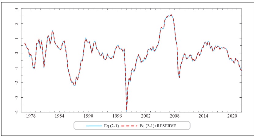
Figure A2.
Equilibrium Real Effective Exchange Rate Misalignments
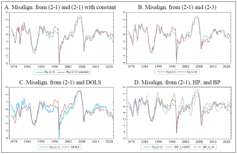
Notes: 1) The figure represents the deviation of the logarithmic real effective exchange rate from the logarithmic equilibrium real effective exchange rate. For convenience, the misalignments are standardized using the mean and standard deviation.
2) Figure A shows the misalignments from equations (2-1) and (2-1) with a constant term.
3) Figure B displays the misalignments from equations (2-1) and (2-3).
4) Figure C shows the misalignments from the OLS and DOLS estimates of equation (2-1), respectively.
5) Figure D indicates the misalignments obtained using Equation (2-1) and the HP filter (smoothing parameter: 16,000) or the bandpass (BP) filter (minimum and maximum cycle periods: pl=6 quarters, pu=32 quarters).
Figure A3.
Cumulative Response Curve (5 variables, lag: 3)
Note: 1)
Figure A4.
Cumulative Response Curve (5 variables, lag: 3, (2-1) with constant term)
Note: 1)
Figure A5.
Cumulative Response Curve (5 variables, lag: 3, (2-2) with constant term)
Note: 1)
Figure A6.
Cumulative Response Curve (5 variables, lag: 3, (2-2))
Note: 1)
Figure A7.
References
-
Ahn, C. 2006. “Natural equilibrium real exchange rate in Korea.”
East Asian Economic Review , vol. 10, no. 2. pp. 47-68. (in Korean)
-
Ambaw, D., M. Pundit, A. Ramayandi, and N. Sim. 2023. “Real exchange rate misalignment and business cycle fluctuations in Asia and the Pacific.”
Asian Economic Journal , vol. 37, no. 2, pp. 164-189.
-
Ambaw, D. and N. Sim. 2021. “Real exchange rate misalignment and civil conflict: Evidence from Sub-Saharan Africa.”
Oxford Economic Papers , vol. 73, no. 1, pp. 178-199.
-
Ball, L. 2012. “Short-run money demand.”
Journal of Monetary Economics , vol. 59, no. 7, pp. 622-633.
-
Bereau, S., A. L. Villavicencio, and V. Mignon. 2012. “Currency misalignments and growth: A new look using nonlinear panel data methods.”
Applied Economics , vol. 44, no. 27, pp. 3503-3511.
-
Bilson, J. 1978. “The monetary approach to the exchange rate-some empirical evidence.”
IMF Staff Papers , vol. 25, pp. 48-75.
-
Bank for International Settlements. June 29, 2009.
BIS 79th Annual Report 2008/2009 . -
Chun, S. E. and C. H. Kim. 2006. “Estimating equilibrium won/dollar real exchange rate: The BEER approach.”
Journal of Economic Studies , vol. 24, no. 2, pp. 1-24. (in Korean) - Clark, P. B. and R. MacDonald. 1998. “Exchange rates and economic fundamentals: A methodological comparison of BEERs and FEERs.” In R. MacDonald and J. Stein. (eds.) Equilibrium exchange rates, Kluwer: Amsterdam. And IMF Working Paper, no. 98/67 (Washington: International Monetary Fund, March 1998).
-
Comunale, M. 2022. “A panel VAR analysis of macro-financial imbalances in the EU.”
Journal of International Money and Finance , vol. 121, no. 102511. -
Christiano, L. J., M. Eichenbaum, and C. Evans. 1996. “The effects of monetary policy shocks: Evidence from the flow of funds.”
Review of Economics and Statistics , vol. 78, pp. 16-34.
-
Christiano, L. J. and T. J. Fitzerald. 2003. “The band pass filter.”
International Economic Review , vol. 44, no. 2, pp. 435-465.
-
Edwards, S. 1989. “Exchange rate misalignment in developing countries.”
The World Bank Research Observer , vol. 4, no. 1, pp. 3-21.
-
Eichenbaum, M and C. Evans. 1995. “Some empirical evidence on the effects of monetary policy shocks on exchange rates.”
Quarterly Journal of Economics , vol. 110, no. 4, pp. 975-1009.
-
Elbadawi, I. A., L. Kaltani and R. Soto. 2012. “Aid, real exchange rate misalignment, and economic growth in Sub-Saharan Africa.”
World Development , vol. 40, no. 4, pp. 681-700.
-
Fidora, M., C. Giordano and M. Schmitz. 2021. “Real exchange rate misalignment in the euro area.”
Open Economics Review , vol. 32, pp. 71-107.
-
Ghura, D. and T. J. Grennes. 1993. “The real exchange rate and macroeconomic performance in Sub-Saharan Africa.”
Journal of Development Economics , vol. 42, no. 1, pp. 155-174.
-
Gnimassoun, B. and V. Mignon. 2015. “Persistence of current-account disequilibria and real exchange-rate misalignments.”
Review of International Economics , vol. 23, no. 1, pp. 137-159.
-
Gnimassoun, B. and V. Mignon. 2016. “How do macroeconomic imbalances interact? Evidence from a panel VAR analysis.”
Macroeconomic Dynamics , vol. 20, no. 7, pp. 1717-1741.
-
Grossmann, A. and A. G. Orlov. 2022. “Exchange rate misalignments, capital flows and volatility.”
The North American Journal of Economics and Finance , vol. 60, no. 101640.https://doi.org/10.1016/j.najef.2022.101640 -
Hodrick, R. and E. C. Prescott. 1997. “Postwar U.S. business cycles: An empirical investigation.”
Journal of Money, Credit, and Banking , vol. 29, no. 1, pp. 1-16.
-
Holtemöller, O. and S. Mallick. 2013. “Exchange rate regime, real misalignment, and currency crises.”
Economic Modelling , vol. 34, pp. 5-14.
-
Kang, S.-M. and S.-Y. Joo. 2004. “Real exchange rate misalignment in Korea, Singapore, and Thailand: Using two different real exchange rates.”
Journal of Money and Finance , vol. 18, no. 2, pp. 1-28. (in Korean) -
Kim. J. S. 1998. “Estimation of Korean won/dollar equilibrium exchange rate.”
Korean Journal of Money & Finance , vol. 3, no. 2, pp. 1-37. (in Korean) -
Klau, M. and S. S. Fung. March 2006. “The New BIS effective exchange rate indices.”
BIS Quarterly Review , pp. 51-65. -
Lee, S. 2016. “The real effective exchange rate of Korean won and economic fundamentals.”
Journal of Finance & Knowledge Studies , vol. 14, no. 2, pp. 127-143. (in Korean) -
Lee, S. and S. Kang. 2022. “The decline in the export impact of the won/dollar exchange rate and its implications.”
i-KIET Industrial Economic Issue , vol. 143, no. 2022-17. KIET. (in Korean) - Lewis, M., A. Martin and G. D. Bella. 2007. Assessing competitiveness and real exchange rate misalignment in low-income countries. IMF Working Paper No. 07/201. International Monetary Fund. Washington, DC.
-
MacDonald, R. 2000. “Concepts to calculate equilibrium exchange rate: An overview.”
Discussion Paper Series 1 , No. 2000.03. Deutsche Bundesbank. Frankfurt. -
Rodrik, D. 2008. “The real exchange rate and economic growth.”
Brookings Papers on Economic Activity , vol. 39, no. 2. pp. 365-439.
-
Park, E.-y. and Y.-J. Kim. 2018. “On the measurement of Korean won/dollar long-run equilibrium exchange rate based on money stock.”
Journal of Economic Studies , vol. 36, no. 2, pp. 125-151. (in Korean)
-
Sekkat, K. 2016. “Exchange rate misalignment and export diversification in developing countries.”
The Quarterly Review of Economics and Finance , vol. 59, pp. 1-14.
-
Sekkat, K. and A. Varoudakis. 2000. “Exchange rate management and manufactured exports in Sub-Saharan Africa.”
Journal of Development Economics , vol. 61, no. 1. pp. 237-253.
- Staehr, K. and R. Vermeulen. 2016. “How competitiveness shocks affect macroeconomic performance across Euro area countries.” ECB Working Paper No. 1940. European Central Bank.
-
Stock, J. and M. Watson. 1993. “A simple estimator of cointegrating vectors in higher order integrated systems.”
Econometrica , vol. 61, no. 4, pp. 783-820.
-
Williamson, J. 1994.
Estimating equilibrium exchange rates . Institute of International Economics. Washington, DC.