

- EAER>
- Journal Archive>
- Contents>
- articleView
Contents
Citation
| No | Title |
|---|
Article View
East Asian Economic Review Vol. 29, No. 1, 2025. pp. 41-76.
DOI https://dx.doi.org/10.11644/KIEP.EAER.2025.29.1.444
Number of citation : 0View
37
Download
33
The Drivers of Inflation in Korea: Insights from a Small Open DSGE Model
|
|
Hongik University |
|---|

Abstract
This study analyzes the drivers of inflation in South Korea using a Dynamic Stochastic General Equilibrium (DSGE) model tailored to the characteristics of Korea as a small open economy. Employing quarterly data from 1999Q2 to 2023Q2, Bayesian estimation is used to estimate Korea-specific parameters. Based on the estimated parameters, impulse response analysis and historical decomposition are conducted. The results indicate that cost-push shocks tied to imported goods pricing have been the primary driver of recent inflation surges in Korea. Accordingly, policymakers need to adopt a comprehensive approach—including not only monetary policy but also macroprudential measures and raw material supply management—to mitigate supply-side inflationary pressures effectively.
JEL Classification: E31, E32, C11, F41
Keywords
Inflation, Dynamic Stochastic General Equilibrium, Bayesian Estimation, Cost-push Shocks
I. Introduction
The annual growth rates of Korea’s Core Consumer Price Index (CPI) exceeded 3.6% and 3.4% in 2022 and 2023, respectively. Although the index declined to 2.2% in 2024, these elevated inflation rates represent unprecedented levels in the past decade.1 Historically, such high inflation rates were observed in the early 2000s (2001–2003) and during the global financial crisis in 2008, when inflation exceeded 3% (Figure 1).
This study identifies the major shocks that have influenced inflation dynamics in Korea since the 2000s. It also investigates the key drivers behind the recent surge in inflation, providing a deeper understanding of the factors contributing to the sharp price increases observed in recent years. Finally, the study explores policy implications for managing interest rate policy effectively to achieve price stability in the context of Korea’s unique economic characteristics.
This study employs the Dynamic Stochastic General Equilibrium (DSGE) model by Justiniano and Preston (2010), which incorporates the characteristics of Korea as a small open economy. Justiniano and Preston (2010) build on the framework of Galí and Monacelli (2005), which assumes imperfect competition and price rigidities, by introducing additional features such as an incomplete asset market, habit formation, and price indexation to past inflation. For the analysis, the study utilizes calibration and Bayesian estimation to estimate Korea-specific parameters. Based on these estimated parameters, the study focuses on inflation, the primary variable of interest, to conduct an in-depth analysis.
The variables used for parameter estimation include Korea’s industrial production, policy interest rate, real effective exchange rate, terms of trade, and core consumer price index (excluding food and energy), as well as the G-7 countries’ industrial production, core consumer price index (excluding food and energy), and average policy interest rate. Quarterly data were utilized, covering the period from 1999Q2 to 2023Q2, which corresponds to the post-IMF crisis era when Korea adopted inflation targeting and transitioned to a floating exchange rate regime.
Based on the analysis of the estimated parameters, during periods of rising prices in the pre-COVID era—when overall inflation was relatively stable—both monetary policy shocks and technology shocks played a significant role in driving inflation in Korea. However, in the two years following 2021, when inflation accelerated sharply, technology shocks continued to contribute substantially, while cost-push shocks emerged as a major influence on price increases. This contrasts with the pre-COVID period, during which cost-push shocks largely helped stabilize inflation; more recently, however, they appear to have propelled inflation upward. These findings indicate that effectively managing supply-side pressures—such as raw material costs and domestic distribution margins—along with fostering productivity growth, is central to maintaining price stability.
While many studies have utilized DSGE models to analyze Korea’s business cycles or optimal monetary policy (considering inflation targeting), few have focused specifically on inflation dynamics and the theoretical transmission channels, as proposed in this study. Analyzing inflation dynamics using a small open economy DSGE model offers the advantage of identifying not only domestic factors but also external factors, such as rising import prices, foreign interest rate shocks, or foreign output fluctuations, that contribute to inflation. This approach is particularly significant for understanding inflation in a highly trade-dependent, small open economy like Korea and represents a valuable contribution to the existing literature.
The remainder of this paper is organized as follows: Section II reviews the existing literature related to this study. Section III describes the model, while Section IV presents the Bayesian estimation results. Section V discusses the findings of the analysis, and Section VI concludes the paper.
1)Global supply chain bottlenecks and heightened energy price volatility have been identified as common factors driving global inflation
II. Literature Review
There is extensive existing research on exchange rate pass-through in Korea. Cha (2007) analyzed the factors driving the increase in Korea's exchange rate pass-through and its impact on domestic inflation. Covering the period from 1980 to 2005, the study examined exchange rate pass-through by different exchange rate regimes. The findings indicated that both short- and long-term exchange rate pass-through to import prices have been increasing, not due to changes in trade composition but rather due to rising pass-through rates at the industry level.
Zhu et al. (2010) used a structural VAR model (including variables such as oil prices, production, exchange rates, money supply, import prices, and consumer prices) to analyze the pass-through effects of won/dollar exchange rate changes. According to their study, the pass-through effects of exchange rate changes on import prices and consumer prices were very small and showed a declining trend over time. They argued that policymakers should prioritize managing inflation over focusing on exchange rates.
Choi (2013) estimated the exchange rate pass-through for Korea’s manufacturing sector in response to changes in the won/dollar exchange rate. Using annual data from 1999 to 2011, a panel analysis was conducted on 30 manufacturing industries. The results showed that a 10% increase in the won/dollar exchange rate led to a 2.4% to 4.9% decrease in dollar-denominated export prices across all industries. The pass-through effect was particularly high in basic materials industries, while industries related to consumer goods—such as food, textiles and apparel, leather products, and miscellaneous manufactured goods—showed minimal responsiveness.
Park and Cha (2014) analyzed the relationship between exchange rate pass-through to consumer prices and monetary policy using panel data from 11 emerging economies that had adopted inflation targeting policies. Their findings indicated that both the level and volatility of inflation decreased following the adoption of inflation targeting. They argued that this reduction in exchange rate pass-through was attributable to monetary authorities effectively managing inflation expectations under the inflation targeting framework.
Lee (2017) estimated the exchange rate pass-through to domestic price levels using a time-varying parameter model with quarterly data. The analysis revealed a general declining trend in exchange rate pass-through since the 2000s. The study found that exchange rate volatility and inflation positively affected exchange rate pass-through, while trade dependency, inflation volatility, and production volatility had negative effects.
Chiang (2021) analyzed the asymmetry and nonlinearity of exchange rate pass-through to import prices across Korean industries. Using the pricing-to-exchange rate model proposed by Goldberg and Knetter (1997), the analysis demonstrated that the pass-through effect was greater during currency appreciations than depreciations, showing significant asymmetry. This effect became more pronounced after the foreign exchange crisis.
Recent studies on DSGE models include Choi (2019), Rhee et al. (2020), Kim et al. (2021), and Hur and Oh (2024). Choi (2019) developed a small open economy DSGE model to analyze Korea’s business cycles and optimal monetary policy. Using Bayesian methods to estimate parameters, the study demonstrated that a positive technology shock leads to an increase in output, a decline in prices, and an appreciation of the exchange rate. In contrast, a positive foreign income shock causes increases in both production and prices. The analysis concluded that the optimal monetary policy rule is one that primarily responds to domestic inflation.
Rhee et al. (2020) developed a small open economy DSGE model to analyze Korea’s business cycles and assess the forecasting performance of macroeconomic variables. Similar to Choi (2019), they estimated the model parameters using Bayesian methods and employed a DSGE-VAR approach. The analysis revealed that, compared to monetary or supply shocks, demand and technology shocks have a more significant impact on key economic variables. This effect was particularly pronounced for growth rates and inflation.
Kim et al. (2021) analyzed the impact of the Federal Reserve’s monetary policy normalization on Korea’s external sector, including exchange rates, capital flows, and swap basis spreads. They conducted scenario analyses focusing on the effects of the Federal Reserve’s tapering and interest rate hikes. Notably, their study shares similarities with the current study in utilizing the model by Justiniano and Preston (2010) to assess the effects of monetary policy normalization on Korea’s exchange rate. The analysis showed that under a pessimistic scenario, the exchange rate could increase by up to 22%, and GDP could initially decline by 2.1% before recovering.
Hur and Oh (2024) employ a DSGE model to examine how the Bank of Korea has conducted monetary policy since the 2000s, showing that it has partially responded to financial stability factors, such as household credit, as well as inflation and growth. Focusing on the perspective of optimizing a central bank’s loss function, they demonstrate that incorporating household debt variables into the interest rate rule leads to more effective medium- to long-term economic stabilization. Consequently, their findings suggest that an Integrated Inflation Targeting framework could serve as a potential alternative for Korea’s monetary policy system.
Previous studies closely related to this research include Choi (2019), Rhee et al. (2020), Kim et al. (2021), and Hur and Oh (2024). Like these studies, the current research is based on a DSGE model but focuses on identifying the theoretical mechanisms through which internal and external factors influence inflation dynamics. Notably, it distinguishes itself from prior research by analyzing the causes of Korea’s recent inflation surge following the COVID-19 pandemic using the DSGE framework.
III. Model
In Chapter III, the DSGE model is briefly described. The model is based on Justiniano and Preston (2010), which builds upon Galí and Monacelli (2005) by introducing assumptions of imperfect competition and price rigidities, along with additional features such as an incomplete asset market, habit formation, and price indexation to past inflation. For a concise explanation of the model, the economy is divided into three agents: households, producers, and retailers (who set prices). The optimal decision-making process for each agent is derived, and the equilibrium, where all markets clear, is defined.
1. Households
Households are assumed to make decisions that maximize their lifetime expected utility.

Household consumption  represents the preference shock for households.
Consumption
where
The household’s budget constraint is given by Equation (3).


 denote, respectively, the overall domestic price level (or consumer price index), the price of domestically produced goods, the domestic currency-denominated price of imported foreign goods, and the foreign currency-denominated price of foreign goods.
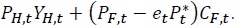
When issuing foreign bonds to borrow from abroad, a risk premium  denotes the risk premium shock.


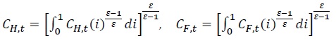
The optimal expenditure allocation condition for domestic goods and foreign goods
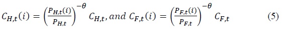
Furthermore, the optimal expenditure allocation condition for the composite of domestic and foreign goods that constitutes the final consumption good is as follows.

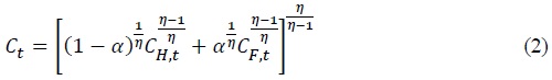
The overall domestic price level (or consumer price index) is defined as: 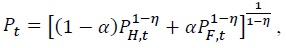 where
where
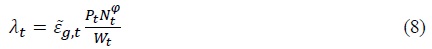
The optimal allocation of expenditure on final consumption goods and labor supply satisfies Equations (7) and (8), respectively.

The allocation of domestic and foreign bonds satisfies the following optimality conditions.
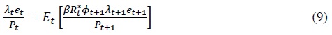
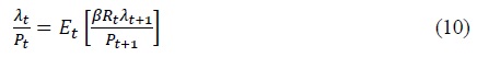
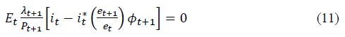
The combination of Equations (9) and (10) yields the Uncovered Interest Rate Parity (UIP) condition.
2. Producers
It is assumed that producers operating in a monopolistically competitive market produce differentiated goods

 Firms that are allowed to set their prices in period
  The Dixit–Stiglitz aggregate price index evolves over time as described in Equation (13).
Firms produce good  represents the technology shock.

In period
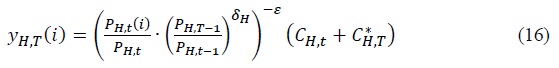
The demand curve is given by Equation (16).
The real marginal cost function for each firm (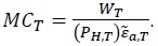
The first-order condition for the firm’s optimization is expressed in Equation (17).

3. Retailers
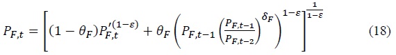
In a monopolistically competitive market, retailers import goods from abroad and set domestic currency prices for these imported goods. Due to this pricing behavior, the Law of One Price does not hold in the short run. Similar to domestic producers, retailers face Calvo-type price rigidity, which allows them to index prices to the inflation rate of the previous period. The Dixit–Stiglitz aggregate price index evolves over time according to Equation (18).
The firm’s price-setting problem in period
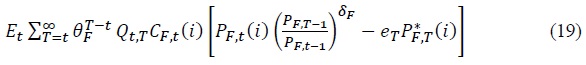
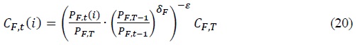
The demand curve for foreign goods that the firm faces is given by Equation (20).
The first-order condition for the retailer’s profit maximization is as follows.
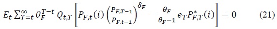
The optimality conditions for the retailers’ pricing problem involve the cost-push shock, indicating that an increase in the cost-push shock leads to a rise in the prices set by retailers for imported goods. This reflects the direct transmission of cost-push shocks to consumer prices through the pricing behavior of retailers, highlighting their role in amplifying supply-side inflationary pressures.
4. Monetary Policy
Monetary policy is conducted following a Taylor rule adapted for a small open economy. In addition to the typical Taylor rule used in closed economies, where interest rates respond to inflation and output, the small open economy version incorporates interest rate responsiveness to exchange rate changes. The parameters

5. Market-Clearing Condition for the Goods Market
The market-clearing condition for the goods market in the domestic economy is as follows.

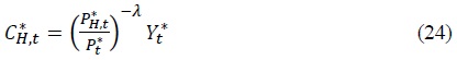
It is assumed that foreign demand for domestically produced goods is determined by Equation (24), and the market clears accordingly. The parameter
6. Foreign Economy and Real Exchange Rate
According to Justiniano and Preston (2010), the foreign economy is assumed to follow a second-order vector autoregressive process for the variables  The real exchange rate (
 Thus, the failure of the Law of One Price implies the existence of a Law of One Price gap (Ψ
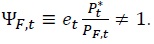
2)Refer to
IV. Estimation
Bayesian estimation is employed to estimate the parameters of the model tailored to Korean data. The estimation uses eight variables: Korea’s industrial production, policy interest rate, real effective exchange rate, terms of trade, core consumer price index (excluding food and energy), G-7 industrial production, G-7 core consumer price index (excluding food and energy), and the average policy interest rate of the G-7. Industrial production and price index data are sourced from the OECD, while policy interest rates and the real effective exchange rate are obtained from the BIS. Korea’s terms of trade are sourced from the Bank of Korea Economic Statistics System. For the G-7 policy interest rates, the average of the seven countries’ rates is used, with Germany, France, and Italy sharing the same Eurozone policy rate.
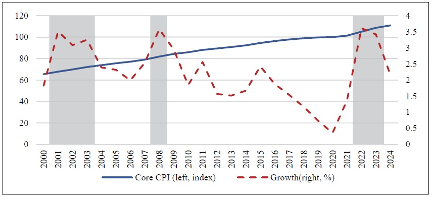
The estimation period spans from May 1999, when Korea adopted inflation targeting and transitioned to a floating exchange rate regime following the IMF crisis, to June 2023. Figure (2) presents the raw data and preprocessed time series of the eight variables used for parameter estimation. Because the calibration parameters rely on quarterly data, we first preprocess the monthly raw data and then calculate quarterly averages, which are used in the analysis.
The dashed line represents the raw data, while the solid line represents the preprocessed data. The left vertical axis indicates the units of the raw data, and the right vertical axis shows the units of the preprocessed data. During preprocessing, trends and seasonality were removed from time series data with such characteristics (e.g., industrial production, terms of trade, and consumer price index).3 For the real effective exchange rate, the data were transformed to align with the model, where an increase corresponds to a depreciation. The policy interest rate was not significantly preprocessed, with only its percentage values converted to decimal form.
Among the eight observable endogenous variables, the primary variable of interest in this study is the consumer price index. Recent consumer price indices for both Korea and the G-7 countries have shown a significant and common increase, representing an exceptionally sharp rise unprecedented during the 25-year analysis period.
The model parameters were estimated using the eight observable endogenous variables. Estimation was carried out in two main steps. First, we conducted an initial mode-searching step to locate the posterior mode for the parameters. Next, we performed Metropolis–Hastings (MH) sampling using a total of 300,000 draws, split into two blocks, discarding the first 20% of draws from each chain as a burn-in period to help ensure convergence. We set the proposal distribution’s scaling factor to 0.3, thereby maintaining a reasonable acceptance rate and effectively exploring the posterior parameter space. Once the sampling was complete, we obtained posterior means and credible intervals for all estimated parameters from the retained portion of the chains.4
The prior distributions for each parameter are based on Justiniano and Preston (2010) and are summarized in Table (1). The shaded areas indicate the mean and standard deviation of the posterior distributions estimated using the data. Parameters not presented in Table (1) were calibrated.5
The estimated means of the parameters are generally similar to the means of the prior distributions, with a few exceptions. However, the standard deviations of the shocks show relatively larger differences, particularly when compared to the standard deviations specified in the prior distributions.6
3)We use time (trend plus a quadratic term) regression to remove the trend, and monthly dummy variables to eliminate seasonal effects, resulting in the cleaned time series.
4)Convergence was evaluated using the Brooks–Gelman R‑hat statistic (Brooks and Gelman, 1998). Out of the 25 parameters estimated, 19 exhibited R‑hat values below 1.1, indicating satisfactory MCMC convergence. For example, the persistence parameter for the cost-push shock had an R‑hat of 1.05, and the largest observed R‑hat among all parameters was 1.28—both of which fall within an acceptable range for ensuring chain stability. The trace plots for seven selected parameters are presented in
5)
6)Three potential reasons can be considered: First, if the standard deviation of the posterior distribution is much smaller than that of the prior distribution, it indicates that the data provides substantial information about the parameters. This suggests that the data strongly influences parameter estimation. Conversely, if the standard deviation of the posterior distribution is much larger than that of the prior, it implies that the model may not fit the data well or that some critical factors might have been omitted. Second, it is possible that the choice of the prior distribution was incorrect or overly restrictive. In such cases, combining the prior with the data to compute the posterior distribution may yield results that differ significantly from the prior distribution. Third, the issue may arise due to problems in the estimation process. The optimization algorithm might not have converged properly, or issues may have occurred during the MCMC sampling process.
V. Results
In Chapter V, impulse response analysis and historical decomposition are conducted based on the estimated parameters. The impulse response analysis provides insights into the effects of each shock on Korea’s consumer price index, while the historical decomposition identifies the factors contributing to inflation dynamics in Korea since 2000. Additionally, the analysis reveals the primary drivers of recent inflation increases and derives relevant policy implications.
1. Impulse Response Analysis
The first set of findings comes from the impulse response functions. In Figure 3 below, we present these functions, calibrated using our estimated parameters, to show how inflation responds to each of the model’s eight shocks. Each panel illustrates the effect on consumer prices (CPI) of a (+) 1 standard deviation shock.
First, the technology shock lowers inflation by nearly 0.7% in the current period, then starts to rebound after about three quarters, eventually fading out. In contrast, the preference shock stimulates demand and raises inflation by around 0.15% during the first one or two quarters, but after that, inflation falls below the baseline and later returns to zero in the medium to long run.
For the monetary policy (interest rate hike) and risk premium shocks, the domestic currency appreciates (i.e., the exchange rate declines), consistent with UIP. Due to this currency appreciation, inflation shows a short-term decline—around 0.12% for monetary policy shocks and about 0.06% for risk premium shocks, occurring either in the current quarter or soon afterward.
The cost-push shock is directly linked to higher prices and exerts a sizable quantitative impact: it raises inflation by more than 0.9% immediately following the shock. Under a one-standard-deviation shock of the same size, the cost-push shock exerts the largest influence on inflation, followed by the technology shock. Finally, foreign output, inflation, and interest rate shocks have a smaller impact relative to domestic shocks, but their effects appear right away and continue to influence inflation over a relatively extended period compared to the other shocks.8
2. Historical Decomposition Analysis
The second main result comes from the historical decomposition shown in Figure 4(a). This analysis reveals the extent to which each shock—technology (epsa), monetary policy (epsm), preference (epsg), risk premium (epsp), cost-push (epsc), foreign output (epys), foreign inflation (epps), and foreign interest rate (eprs)—has contributed to Korean inflation fluctuations since 2000.
According to our historical decomposition, apart from the most recent five years, Korea’s inflation had been relatively stable. During periods of rising prices (beginning around the 40th quarter of the sample, i.e., following the global financial crisis), monetary policy shocks (epsm) and technology shocks (epsa) played a major role in driving inflation higher. However, in the last two years—roughly from 2022 through the final six quarters of the sample—technology shocks (epsa) continued to have a significant impact on inflation, while cost-push shocks (epsc) emerged as a central driver of rising prices. Notably, cost-push shocks had previously helped stabilize inflation, but they now contribute in the opposite direction, representing a new finding.
Figures 4(b) and 4(c) illustrate historical decompositions for domestic goods inflation and imported goods inflation, respectively. As shown in (c), cost-push shocks have been fueling the recent surge in import prices. Consequently, the inflation upturn does not stem solely from domestic producer prices but also from higher inflation in imported items. Through cost-push shocks, import price increases raise domestic inflation overall.
Looking at the variance decomposition confirms that cost-push shocks (epsc) account for about 63% of inflation (pie) fluctuations, followed by technology shocks (epsa) at around 30%. By contrast, monetary policy (epsm) and preference (epsg) shocks contribute only about 3%, while foreign inflation (epps) and foreign interest rate (eprs) shocks explain almost 0%. This suggests that, rather than directly capturing external pressures through shocks like foreign inflation (epps), the rise in external costs is strongly passed through to Korean prices via retailers’ pricing decisions (the cost-push channel). In other words, domestic inflation is heavily influenced by supply-side factors (e.g., import raw materials and distribution margins) and productivity shifts, whereas the model’s separate foreign inflation and interest rate shocks appear to exert a relatively small direct effect.9
Since 2022, cost-push shocks have come to the forefront in driving inflation higher, due to soaring costs of commodities and supply chains under COVID-19, the Russia–Ukraine war, and heightened global economic uncertainty. In particular, geopolitical tensions and pandemic-related bottlenecks have pushed up energy and raw material prices, placing strong upward pressure on domestic inflation. Thus, what had been relatively moderate cost-side pressures pre-COVID can become amplified amid significant global instability, making cost-push shocks a key factor in recent changes to inflation.
Bringing together these historical decomposition findings, the policy implication is that monetary policymakers should closely monitor and respond to external supply costs (e.g., import prices), domestic wage and distribution costs, and technological factors. Previously, cost-push shocks contributed to stable inflation or had a limited effect under relatively moderate price pressures; however, they have recently shifted to driving price increases through surging import prices and other external supply-side fluctuations. Therefore, it is crucial to manage and predict global raw material and energy prices as well as domestic distribution costs in a more proactive way.
Furthermore, as the contribution of technology shocks (epsa) expands, there is a need to support long-term sustainable growth in the real sector—such as by improving productivity—and also to minimize the inflationary impact of unexpected technological changes through policy measures (for example, linking R&D investment to restructuring policies). Finally, examining the results of the historical decomposition reveals that monetary policy has exerted a relatively larger influence during periods of rising prices than when prices were declining. In light of this, relying solely on policy rate adjustments may not be sufficient during inflationary phases. Therefore, to prevent supply-side pressures and surging import prices from spilling over into broader inflation, it is advisable to employ a range of tools in tandem, including macroprudential and exchange-rate policies.
8)While the impact of the foreign output shock on inflation is relatively larger than that of foreign interest rate or foreign inflation shocks, it remains relatively modest compared to the non-foreign shocks. For additional responses of other variables to each shock, please refer to
9)Although the overall quantitative contribution of monetary policy shocks to inflation appears relatively small over the entire period, their effect during episodes of rising inflation seems significant. In other words, monetary policy tends to have an asymmetrical impact on inflation, exerting a stronger influence when prices are on the upswing compared to when they are declining.
VI. Conclusion
This study aims to identify the key shocks that have influenced Korea’s inflation dynamics since the 2000s. By examining these factors, it seeks to uncover the main drivers behind the recent surge in inflation. Furthermore, the analysis focuses on deriving policy implications for the effective operation of interest rate policies to ensure price stability in the face of these inflationary pressures.
The analysis reveals that during the pre-pandemic period, when inflation overall remained relatively stable, the occasional price upswings were primarily attributable to monetary policy shocks and technology shocks. However, over the last two years since 2022, during which inflation surged more sharply, technology shocks still played a prominent role while cost-push shocks emerged as a key driver of rising prices. Interestingly, whereas cost-push shocks had previously helped contain inflation, they are now pushing it upward. These findings underscore that properly managing supply-side burdens—such as raw material costs and domestic distribution margins—while encouraging productivity growth is central to achieving price stability.
This study uses the small open economy DSGE framework of Justiniano and Preston (2010), estimated with Korean quarterly data, to shed light on the key factors behind recent inflation. While this approach provides valuable insights, it inherits certain limitations of the model. In particular, it lacks a fiscal block, making it less suitable for analyzing the effect of revenue and spending changes on higher inflation. It also simplifies external channels (e.g., foreign interest rates and inflation), which may underrepresent the role of global shocks in a small open economy. Addressing these constraints and developing a more refined model—one that integrates both domestic fiscal policy and external financial channels—remains an important avenue for future research.
Tables & Figures
Figure 1.
Core Consumer Price Index(CPI) in Korea: Year 2000~2024
Note: Core Consumer Price Index(CPI) represents a measure of inflation that excludes volatile prices like food and energy from the CPI.
Source: Bank of Korea Economic Statistics System
Figure 2.
Time Series Data Used for Parameter Estimation
Figure 2.
Continued
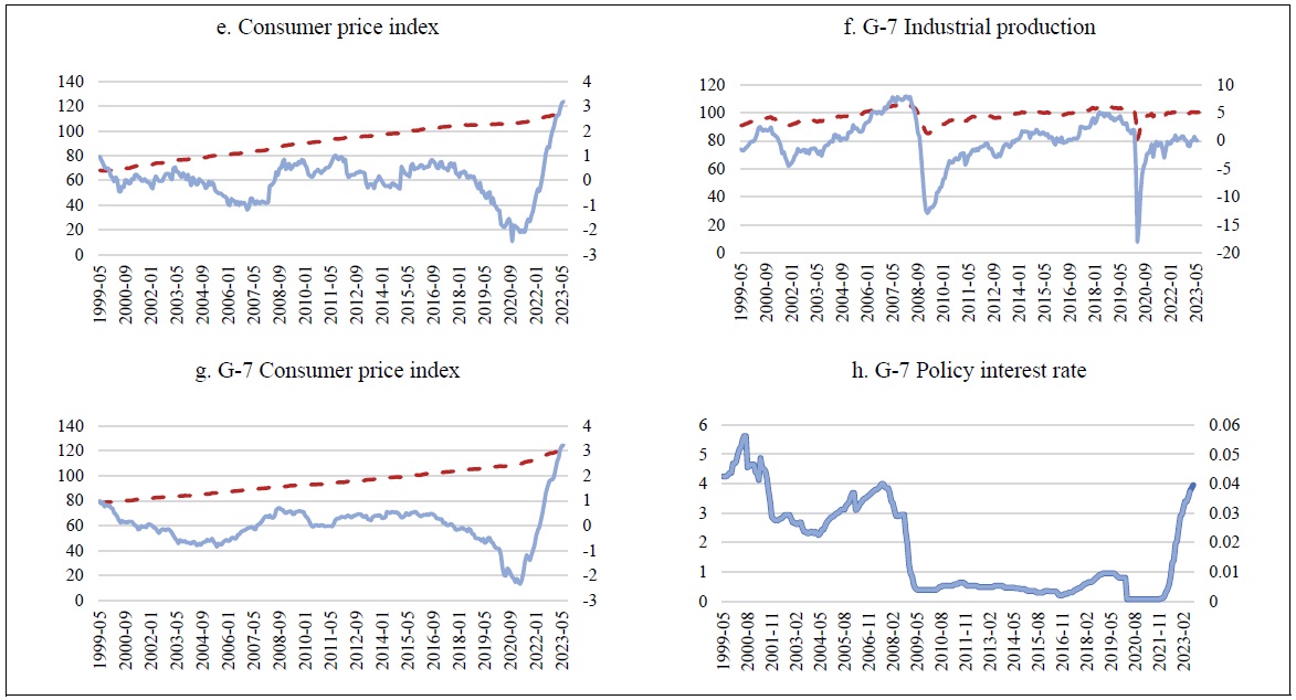
Note: The dashed lines represent the raw data(left y-axis), while the solid lines represent the preprocessed data(right y-axis). Consumer price indices for Korea and the G-7 exclude food and energy.
Source: Author’s calculation based on data from the OECD, BIS, and the Bank of Korea Economic Statistics System.
Table 1.
Prior and Posterior Distributions of Parameters
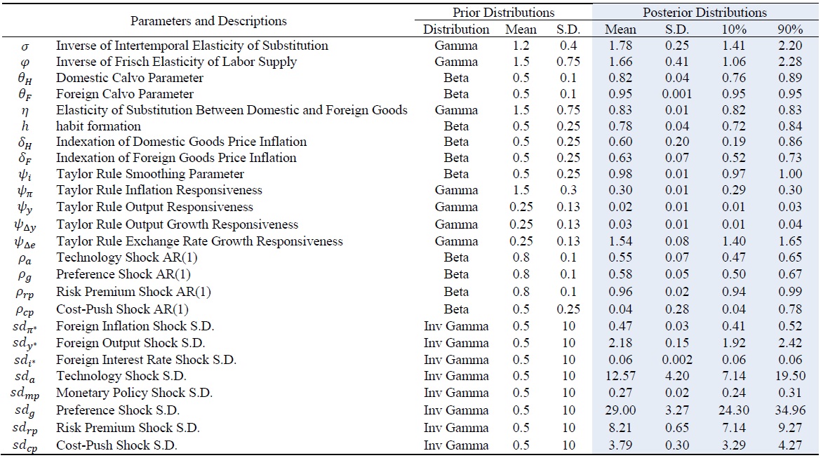
Source: Author’s calculation based on
Figure 3.
Impulse Response Functions of Inflation to Eight Shocks
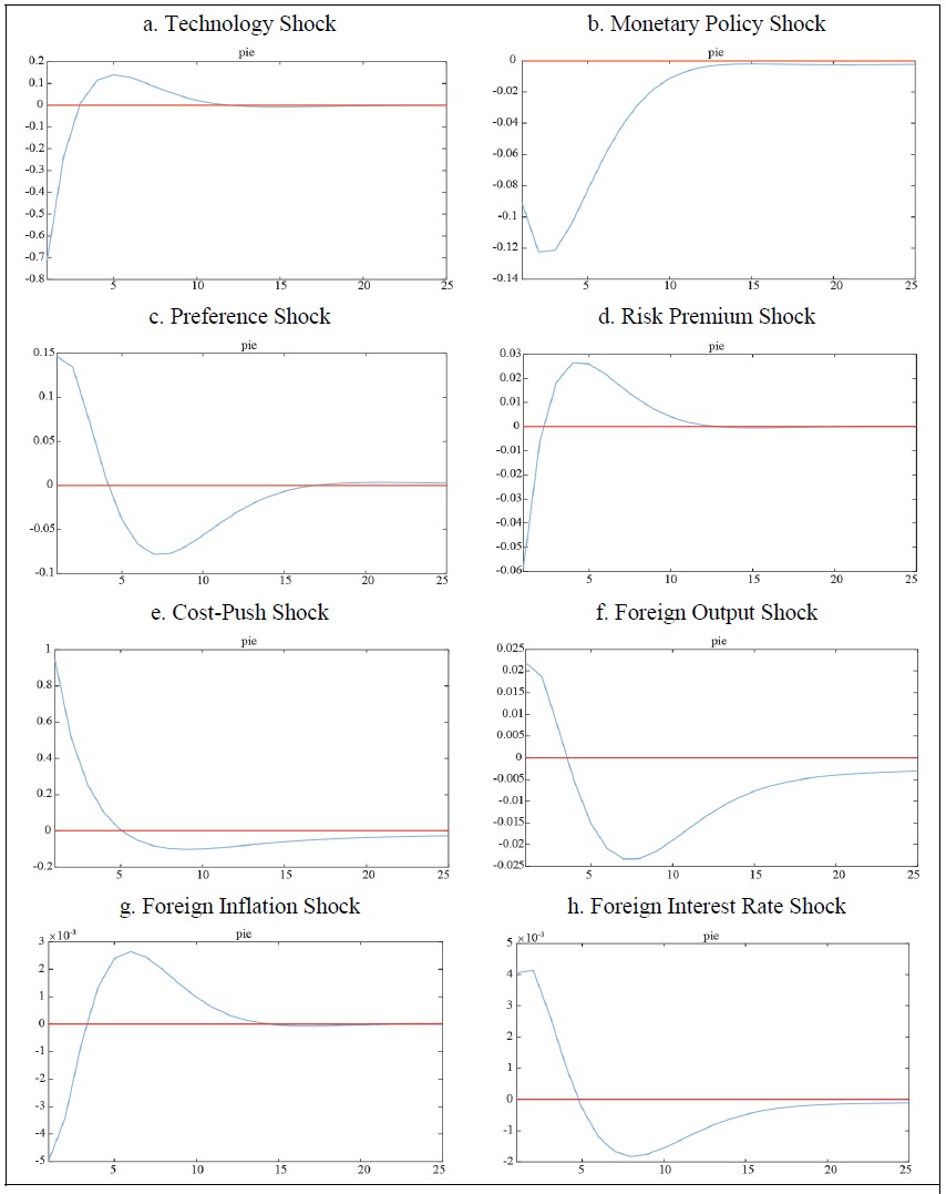
Source: Author’s calculation.
Figure 4.
Historical Decomposition of Korea’s Inflation
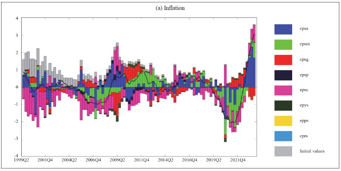
Figure 4.
Continued
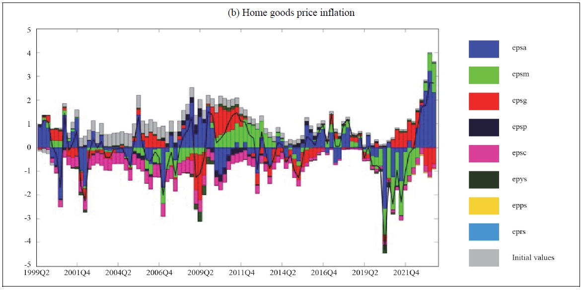
Figure 4.
Continued
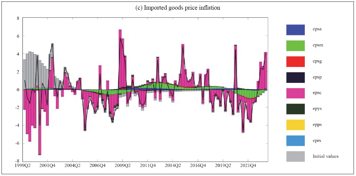
Note: epsa = technology shock, epsm = monetary policy shock, epsg = preference shock, epsp = risk premium shock, epsc = cost-push shock, epys = foreign output shock, epps = foreign inflation shock, eprs = foreign interest rate shock. The solid line represents Korea’s consumer price index with trends and seasonality removed.
Source: Author's calculation.
Appendix Figure 1.
Diagnostic Trace Plot for Selected Parameters
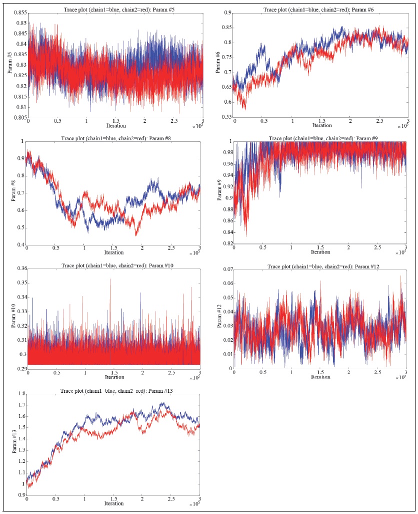
Note: Parameter #5, 6, 8, 9, 10, 12, and 13 correspond to the trace plots for the
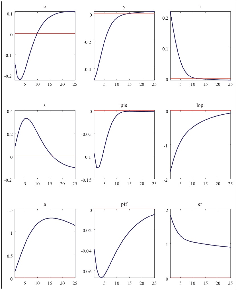
Appendix Figure 2.
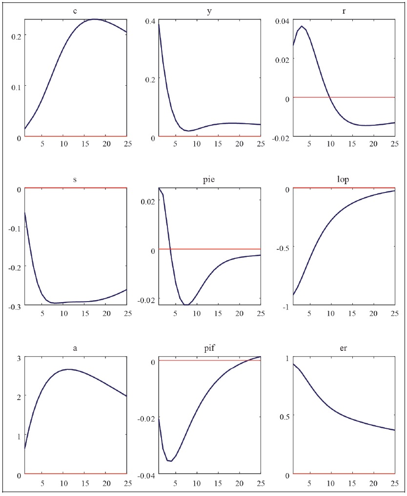
Impulse Response Functions to Technology Shocks
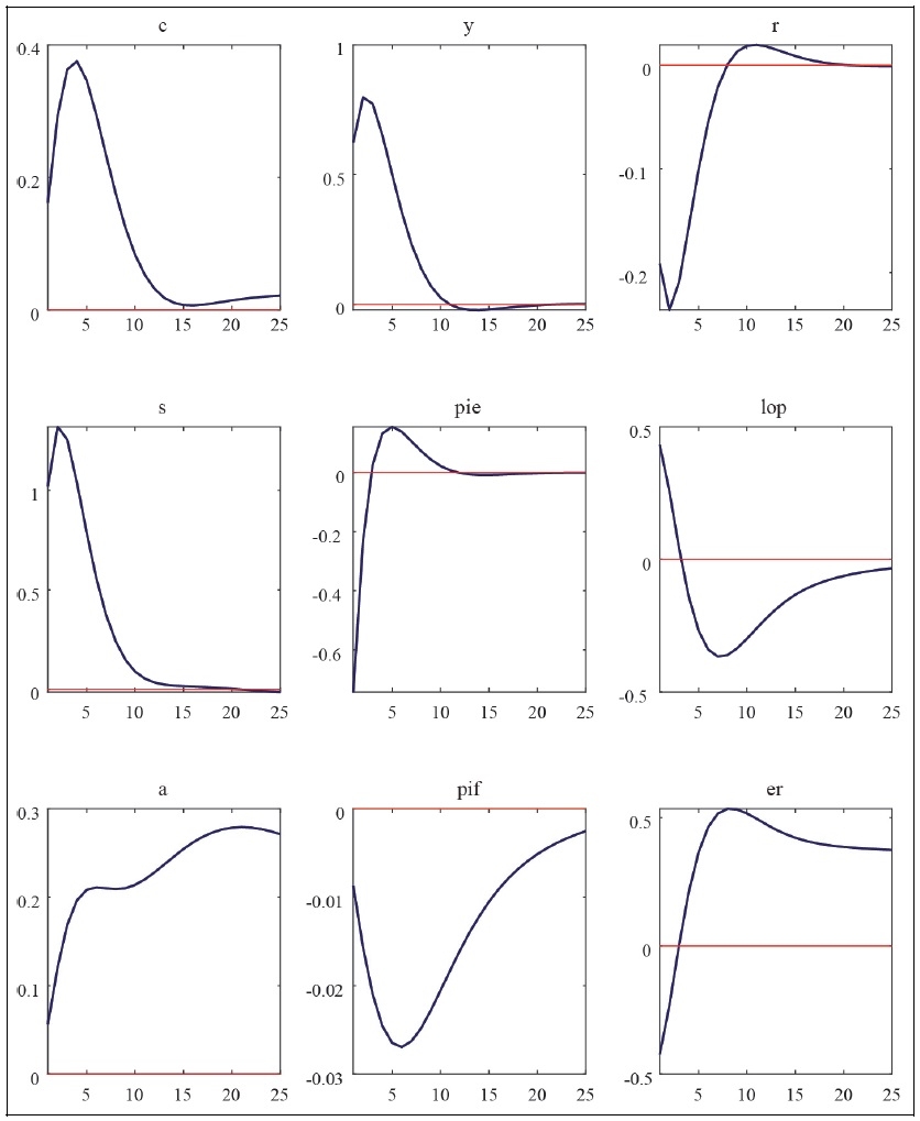
Note: c = consumption, y = GDP, r = policy interest rate, s = terms of trade, pie = CPI inflation rate, lop = law of one price gap, a = net foreign asset position, pif = imported goods price, er = exchange rate.
Source: Author’s calculation.
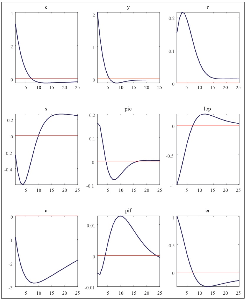
Appendix Figure 3.
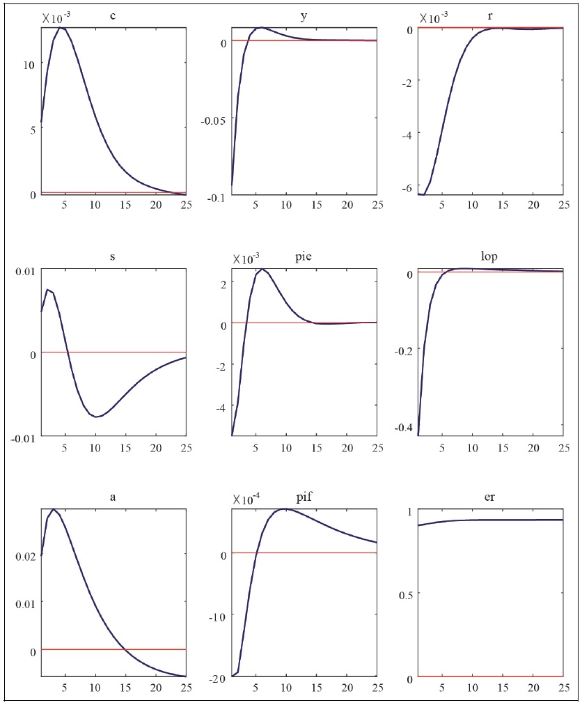
Impulse Response Functions to Monetary Policy Shocks
Note: c = consumption, y = GDP, r = policy interest rate, s = terms of trade, pie = CPI inflation rate, lop = law of one price gap, a = net foreign asset position, pif = imported goods price, er = exchange rate.
Source: Author’s calculation.
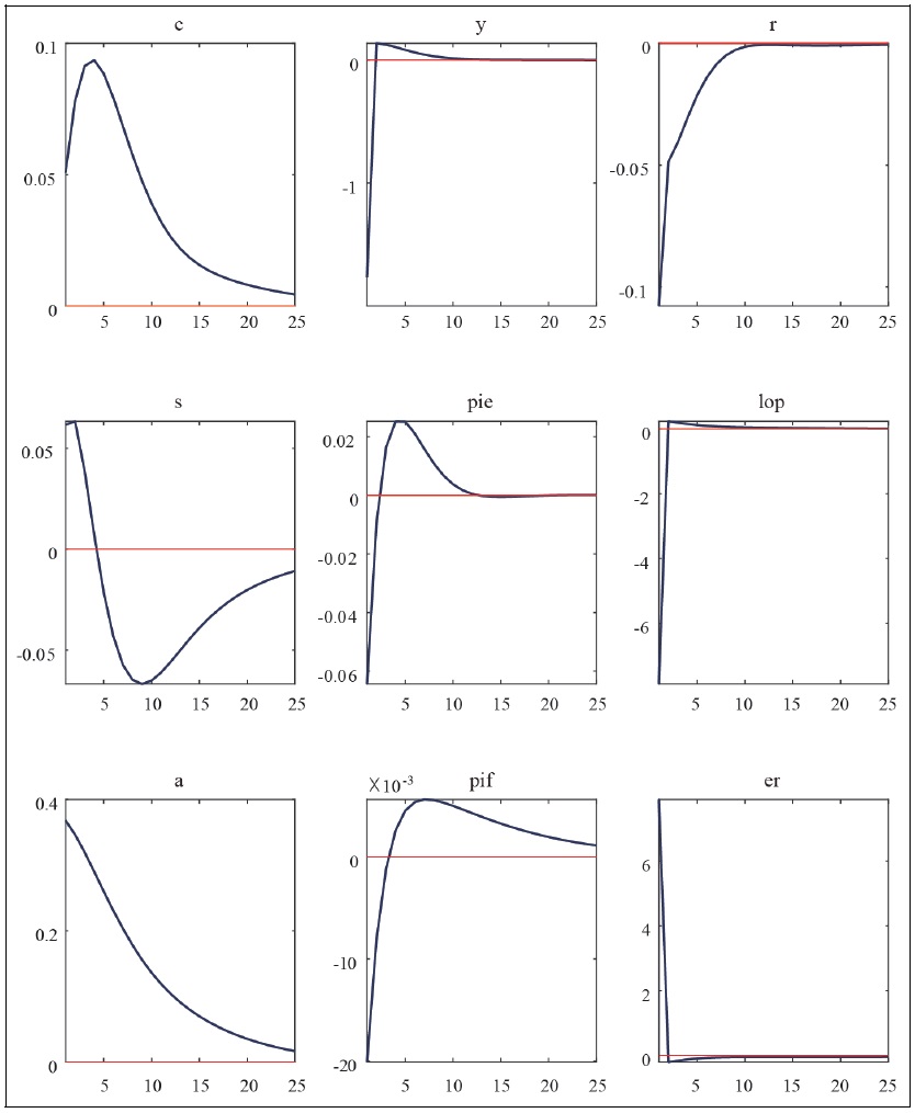
Appendix Figure 4.
Impulse Response Functions to Preference Shocks
Note: c = consumption, y = GDP, r = policy interest rate, s = terms of trade, pie = CPI inflation rate, lop = law of one price gap, a = net foreign asset position, pif = imported goods price, er = exchange rate.
Source: Author’s calculation.
Appendix Figure 5.
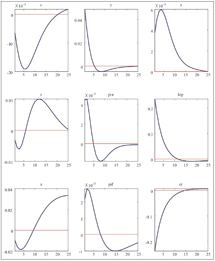
Impulse Response Functions to Risk Premium Shocks
Note: c = consumption, y = GDP, r = policy interest rate, s = terms of trade, pie = CPI inflation rate, lop = law of one price gap, a = net foreign asset position, pif = imported goods price, er = exchange rate.
Source: Author’s calculation.
Appendix Figure 6.
Impulse Response Functions to Cost-push Shocks
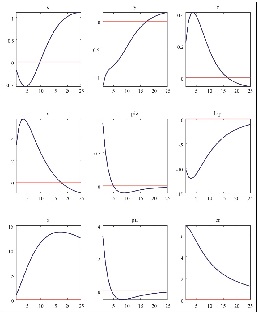
Note: c = consumption, y = GDP, r = policy interest rate, s = terms of trade, pie = CPI inflation rate, lop = law of one price gap, a = net foreign asset position, pif = imported goods price, er = exchange rate.
Source: Author’s calculation.
Appendix Figure 7.
Impulse Response Functions to Foreign Output Shocks
Note: c = consumption, y = GDP, r = policy interest rate, s = terms of trade, pie = CPI inflation rate, lop = law of one price gap, a = net foreign asset position, pif = imported goods price, er = exchange rate.
Source: Author’s calculation.
Appendix Figure 8.
Impulse Response Functions to Foreign Inflation Shocks
Note: c = consumption, y = GDP, r = policy interest rate, s = terms of trade, pie = CPI inflation rate, lop = law of one price gap, a = net foreign asset position, pif = imported goods price, er = exchange rate.
Source: Author’s calculation.
Appendix Figure 9.
Impulse Response Functions to Foreign Interest Rate Shocks
Note: c = consumption, y = GDP, r = policy interest rate, s = terms of trade, pie = CPI inflation rate, lop = law of one price gap, a = net foreign asset position, pif = imported goods price, er = exchange rate.
Source: Author’s calculation.
References
-
Benigno, P. 2009. “Price Stability with Imperfect Financial Integration.”
Journal of Money, Credit and Banking , vol. 41 (SUPPL. 1), pp. 121-149.
-
Cha, H. K. 2007. “Analysis on the Increase of Import Price Exchange Rate Pass-Through.”
Journal of Economic Studies , vol. 25, no. 4, pp. 205-230. -
Chiang, B. G. 2021. “Asymmetric and Nonlinear Exchange Rate Pass-Through to Import Prices in Korea.”
Journal of Economic Studies , vol. 39, no. 3, pp. 37-59. 10.30776/JES.39.3.2
-
Choi, Y.-J. 2013. “The Estimation of Exchange Rate Pass-through on Korean Export Price Using Panel Data.”
Journal of International Trade & Commerce , vol. 9, no. 3, pp. 105-129.
-
Choi, Y.-J. 2019. “The Analysis of Business Cycle and Monetary Policy under the Incomplete Exchange Pass-through.”
International Area Studies Review , vol. 23, no. 4, pp. 267-291. -
Galí, J. and T. Monacelli. 2005. “Monetary Policy and Exchange Rate Volatility in a Small Open Economy.”
The Review of Economic Studies , vol. 72, no. 3, pp. 707-734.
-
Goldberg, P. K. and M. M. Knetter. 1997. “Goods Prices and Exchange Rates: What Have We Learned?”
Journal of Economic Literature , vol. 35, no. 3, pp. 1243-1272. -
Hur, J. and H. S. Oh. 2024. “Optimal Monetary Policy System for Both Macroeconomics and Financial Stability.”
KDI Journal of Economic Policy , vol. 46, no. 1, pp. 91-129. -
International Monetary Fund. 2021.
World Economic Outlook: Recovery during a Pandemic—Health Concerns, Supply Disruptions, Price Pressures . Washington, DC: Internation Monetry Fund. -
Justiniano, A. and B. Preston. 2010. “Monetary Policy and Uncertainty in an Empirical Small Open-Economy Model.”
Journal of Applied Econometrics , vol. 25, no. 1, pp. 93-128.
- Kim, N., Kim, H., and H. Park. 2021. “The Effects and Implications of the U.S. Monetary Policy Normalization.” KIF Policy Analysis Report 2021(2), pp. 1-116.
-
Kollmann, R. 2002. “Monetary Policy Rules in the Open Economy: Effects on Welfare and Business Cycles.”
Journal of Monetary Economic s, vol. 49, no. 5, pp. 1017-1023. -
Lee, S. 2017. “The Effects of Macroeconomic Fundamentals on Exchange Rate Passthrough.”
Journal of Finance and Knowledge Studies , vol. 15, no. 2, pp. 55-78. -
McCallum, B. and E. Nelson. 2000. “Monetary Policy for an Open Economy: An Alternative Framework with Optimizing Agents and Sticky Prices.”
Oxford Review of Economic Policy , vol. 16, no. 4, pp. 74-91.
-
Monacelli, T. 2005. “Monetary Policy in a Low Pass-through Environment.”
Journal of Money, Credit and Banking , vol. 37, no. 6, pp. 1047-1066.
- Oh, K., Kim, Y., Lee, J., and J. Kang. 2022. “Assessment of Inflationary Pressure Trends.” BOK Issue Note No. 2022-1, pp. 1-8.
-
Park, S. Y. and H.-K. Cha. 2014. “The Relationship Between Inflation Targeting and the Pass-through of Exchange Rate into CPI in Emerging Markets.”
The Journal of Korean Public Policy , vol. 16, no. 4, pp. 185-206. -
Rhee, J.-H., Sung, M.-K., and J. S. Lee. 2020. “Study on Macroeconomic Forecasting Power Using Bayesian DSGE Model.”
Korean Jouranl of Business Administration , vol. 33, no. 3, pp. 413-441. -
Schmitt-Grohé, S. and M. Uribe. 2003. “Closing Small Open Economy Models.”
Journal of International Economics , vol. 61, no. 1, pp. 163-185.
-
Zhu, S., Lee, M. H., and K. S. Hwang. 2010. “The Exchange Rate Pass-through Effects on Korean Import and Consumer Prices Using a Structural VAR Model.”
Journal of Economic Studies , vol. 28, no. 2, pp. 85-108.