

- EAER>
- Journal Archive>
- Contents>
- articleView
Contents
Citation
| No | Title |
|---|
Article View
East Asian Economic Review Vol. 29, No. 3, 2025. pp. 337-369.
DOI https://dx.doi.org/10.11644/KIEP.EAER.2025.29.3.452
Number of citation : 0View
47
Download
37
Business Cycles in Korea: Insights from a TANK Model
|
|
Kyung Hee University |
|---|---|
|
|
Kyung Hee University |

Abstract
This paper sets up a medium-scale small open economy TANK model with incomplete markets to address business cycles in Korea extensively. The estimated model via Bayesian estimation methodology shows that the fraction of households who lack access to financial markets increased from 30 percent to 40 percent after the Asian Financial Crisis. This feature appears to be associated with structural changes in employment practices, including life-time employment and seniority-based salaries, as well as an increase in part-time jobs after the crisis. Since the mid-1970s, domestic markup, government spending, and risk premium shocks have been key factors influencing business cycles in Korea.
JEL Classification: E32, F31
Keywords
Bayesian Estimation, Business Cycles, Constrained Households, TANK Model
I. Introduction
Although the so-called New Keynesian model, or neo-classical synthesis, has dominated macroeconomics, macroeconomists have attempted to construct macroeconomic models solely in terms of aggregates by carefully arranging complete markets and the initial distribution of wealth, thereby keeping the distribution of wealth from affecting aggregates such as prices and outputs. Nevertheless, a growing body of literature on the heterogeneous-agent New Keynesian (HANK) model has challenged our assumption that heterogeneity in income and consumption may not impact the dynamics of aggregates and the interplay of monetary and fiscal policy during economic cycles.
Kaplan et al. (2018), Auclert (2019), and Auclert et al. (2024a, 2024b) show that the HANK models that incorporate market incompleteness, heterogeneity in the form of idiosyncratic risk and their feedback effects to aggregates are successful in addressing aggregate fluctuations as well as their interaction between inequality and monetary and fiscal policy as in the data. However, the lack of analytical tractability and transparency associated with HANK models makes it non-trivial to solve the dynamics of HANK models with a time-varying wealth distribution and uncover the sources and driving forces of business cycles.
In this respect, the two-agent New Keynesian (TANK) models with simple heterogeneity in households are well-suited for analyzing and measuring the effects of market incompleteness and heterogeneity on aggregate variables. The earlier literature on two-agent models addressing the business cycle has highlighted the importance of differences in access to financial markets in influencing the impact of monetary and fiscal policy transmission.
Although the simple TANK model with hand-to-mouth (HtM) households does not allow for any idiosyncratic shocks and an endogenous fraction of constrained households, Debortoli and Gali (2018) demonstrate that the tractable TANK model is capable of approximating the dynamics of the HANK model with similar redistribution schemes.1
The feature of a small open economy TANK model is very tractable in that it is isomorphic to the open economy RANK model. For example, the simple open economy TANK model consists of five equations, similar to the RANK model: the NKPC, the goods market clearing condition, the aggregate demand equation, the risk sharing condition, and the monetary policy equation. However, a close examination of the equilibrium conditions of the TANK and RANK models reveals starkly different features in them. Contrary to the RANK model, the share of HtM households affects both the aggregate demand equation and the NKPC in a TANK model. Furthermore, since HtM households lack access to financial markets, the consumption of unconstrained households that share risks with foreign unconstrained households matters to the equilibrium exchange rate.
Regarding business cycles in Korea, there are some noteworthy papers. Jung (2019) establishes a simple TANK model comprising three equations to examine the role of HtM households in business cycles in Korea. Lee et al. (2023) make one step further to set up a small open economy HANK model with nominal price and wage rigidities to explore the role of income inequality in Korean business cycles. Moreover, Jung (2024) analyzed basic economic shocks in a simple Tank model, namely domestic productivity shocks, foreign productivity shocks, and monetary shocks. The previous studies have emphasized the significance of taking into account the existence of a significant portion of economically marginalized households when examining the factors driving business cycles in Korea.
In this paper, we will address the following questions by estimating the fraction of HtM households in Korea with a small open economy TANK model. How does the fraction of economically neglected households (HtM households) shape business cycles in Korea? Has the proportion of HtM households in Korea who lack access to financial markets changed significantly over time, i.e., between a high economic growth era (before the 1997 Asian Financial Crisis) and a low economic growth era with the ongoing Great Moderation period (after the 1997 Asian Financial Crisis)? What kind of shocks have been the main driving forces in business cycles in Korea since the mid-1970s?
For this purpose, we set up a two-block small open economy TANK model with a relatively simple heterogeneity as in Bilbiie (2008), Debortoli and Gali (2018), Gali et al. (2007) and Jung (2024). We estabilish a small open economy medium-scale TANK model with various shocks. We estimate some deep parameters of the model using quarterly data spanning from 1976:3Q to 2018:3Q, employing Bayesian estimation methods. Finally, we assess the relative significance of each shock and the importance of financial frictions throughout the business cycle. In particular, we split the sample periods into two subsample periods to examine at how the share of HtM households had varied before and after the 1997 Asian Financial Crisis, which paved the way for economic structural reforms and economic policy changes such as flexible exchange rates regime, adoption of an inflation targeting policy and a shift in employment practices including life-time employment and seniority-based salaries.
Several results are worth highlighting.
First, a substantial fraction of households in Korea is financially constrained. The estimated fraction of constrained households is approximately 0.32 in the first subsample periods, running from 1976:3Q to 1997:2Q, a value comparable to the estimate in Jung (2019), which employs the maximum likelihood methodology. Furthermore, more households are limited in their asset participation in financial markets after the Asian Financial Crisis, i.e., in the second subsample periods, running from 1993:3Q to 2018:3Q. The fraction of constrained households in Korea has increased to 0.4. This feature partly reflects the structural changes in life-time employment and seniority-based salaries in the labor market, an increase in unstable part-time after the crisis, and the negative effect of the enduring Great Recession on the Korean economy.
Second, domestic markup and government shocks have significantly contributed to variations in output before and after the Asian Financial Crisis. The dominant contribution of a government spending shock to output fluctuations in the second subsample period reflects the features of the world-wide Great Recession, during which the effectiveness of conventional monetary policy is limited. The domestic productivity shock has substantially contributed to the variations in output during the high economic growth era, i.e., in the first subsample period. However, its contribution to output fluctuations is very limited during slow economic growth and recessionary periods, i.e., after the Asian Financial Crisis.
Third, the monetary policy shock has dominated variations of inflation before and after the Asian Financial Crisis. However, the monetary policy shock was less volatile in the second subsample period, during which the Korean economy successfully transformed its structures to be more resilient, and the Bank of Korea implemented a more systematic and transparent monetary policy in the inflation-targeting era.
Finally, the risk premium, or country spread, has played a dominant role in variations of output and inflation after the Asian Financial Crisis, as a world-wide enduring and prevalent Great Recession affected the world economy in the era of globalization.
The remainder of the paper is organized in four sections. Section II sets up a canonical two-agent New Keynesian model. Section III addresses the quantitative implications of the model. Section IV concludes.
1)Bilbiie (2019, 2020) expands a basic TANK model into a manageable two agent heterogeneous agent model with idiosyncratic shock to examine the impact of monetary and fiscal policies on consumption and output.
II. Model
There is a fraction 1 −
1. Households
The preferences are assumed to be common across all households with the same discount factor
(1) Unconstrained households
An unconstrained household maximizes an intertemporal utility function given by
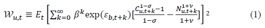
subject to a sequence of budget constraints. Here 

where

Here,
Assuming that domestic unconstrained households can trade both home and foreign risk-free one-period nominal bonds  unconstrained household’s budget constraint can be expressed as
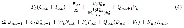
where  are the interest rates corresponding to the bonds, respectively. The function
  incorporates the cost or risk premium associated with international borrowings. The risk premium, represented by
  increases with the country foreign debt, as indicated by
 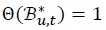 in the steady state where
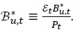
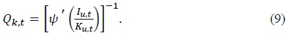
The capital accumulation equation is given by
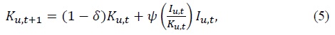
where  denotes the capital adjustment cost with
The optimization condition of unconstrained households is given by

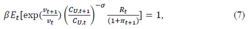

where 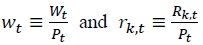 denote the real wage and the real rental cost of capital at time
Notice that first-order conditions for the unconstrained domestic and foreign household imply that the equilibrium real exchange rate

where the asterisk (*) indicates the foreign variable corresponding to the domestic variable. The risk-sharing condition in Equation (10) for an incomplete market can be log-linearized around the steady-state as follows:
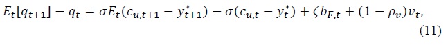
where  and
and  represents the log approximation of the corresponding variable
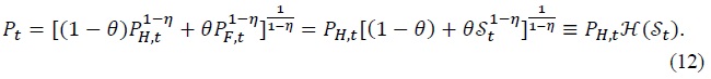
  Notice that the CPI can be expressed in terms of the domestic price index (DPI) and terms of trade
  as follows:
(2) Constrained households
Constrained or HtM households lack access to financial markets. They just supply labor

where
HtM household’s optimization conditions can be written as

and the budget constraint (13).
2. Domestic Firms
Assume that there is a continuum of firms indexed by 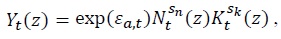 where exp(
Under the assumption of perfectly competitive input markets,
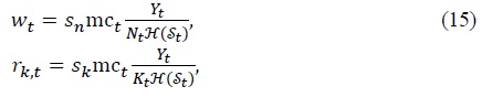
where  and
and
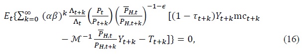
Following Calvo (1983) and Yun (1996), domestic firm  to maximize its present discount value of profits with a probability (1 −
  is the same for the reoptimizing firms, i.e.,
 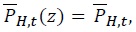 the reoptimized price setting condition can be written as
where Λ represents the steady-state average markup in the domestic goods market.
Denoting  the domestic price aggregator can be represented in terms of the relative price
  as
as

where  is the DPI inflation rate at time
3. Importing Firms
For the sake of simplicity, we assume that the Law of One Price holds for all individual imported goods for all time. Then, the price of foreign good  with a converting factor

A small weight is given to consumption goods produced in a small economy(
4. Monetary Authority
Assume that both the domestic and foreign monetary authorities implement a typical Taylor interest rate rule as follows:


where  respectively. The domestic and foreign monetary authorities are assumed to set non-negative coefficients
5. Aggregation
Aggregate consumption and aggregate hours are given by


Aggregate dividend, capital, investment, and bond holdings also satisfy


Finally, the aggregate share-holdings satisfy
6. The Rest of the World
The rest of the world economy can be represented by a standard closed economy New Keynesian model consisting of households, firms, and fiscal and monetary authorities. We assume that the monetary authority in the rest of the world implements a typical Taylor rule.
Without spelling out the explicit representation of each sector in a foreign country, we assume that there is an aggregate demand shock in the form of preference shock (


The rest of the equilibrium conditions, which can be represented by the standard ones in a closed economy, are not discussed in the paper.
7. Equilibrium
Aggregating individual output across firms yields the aggregate output
where 
Assuming a symmetric degree of home bias across countries with the home country’s relative size being insignificant, goods market clearing in the home country with a government spending

The competitive equilibrium conditions include the efficiency conditions and budget constraints of households and firms, as well as the market clearing conditions for goods, labor, equity, money, and bond markets.
2)For
III. Estimation
In this section, we will estimate the key parameters, such as the fraction of constrained households, to assess the contribution of the main driving forces of business cycles in Korea using a small open economy TANK model specified in the previous section.
1. Dynamics around Steady State
In this subsection, we present the log-linearized equilibrium conditions of the small country, focusing on small fluctuations of the endogenous variables around the steady state , similar to the approach used in the large economy.
The IS-curve type Euler equation in the small economy can be log-linearized around the steady state as

while the unconstrained and constrained households’ optimization conditions for hours can be expressed as


The goods market clearing condition and the budget constraint of constrained households can be written as


where

where  and
and


Domestic household’s choice of capital and investment and the law of motion for capital can be log-linearized as follows:


while the aggregate production can be written as

Here


The international risk-sharing condition implies that the real exchange is proportional to the relative domestic and foreign consumption of unconstrained households.3
Here, the net asset holdings are related to the exports as follows:

The definition of the real exchange rate, the terms of trade, and the definition of the CPI yield a close relationship among them as follows:


Finally, a Taylor rule can be written as follows.

Note that we put (1 +
Domestic preference, productivity, investment, capital, exogenous spending, and markup shocks, except monetary shock, follow an AR(1) process as follows.

where  for
for
Equation (32)-(50) determine 19 endogenous variables  given domestic exogenous variables
  and the evolution of the endogenous and exogenous variables of the rest of the world
2. Calibration
We estimate the model presented in the previous section with Bayesian estimation techniques using six key macro-economic quarterly Korean time series from 1976:3Q to 2018:4Q as observable variables: the log of real GDP, the log of real consumption, the log of terms of trade, the log of the GDP deflator, the log of the CPI, and a call rate. All variables are HP-filtered before applying Bayesian estimation methods. As the data lack sufficient information to estimate all parameters of the TANK model, it is necessary to fix a subset of the model's parameters before conducting the estimation.
All parameter values calibrated in this paper are listed in Table 1. First, the degree of goods market openness (
3. Estimation Results
Since the large economy is exogenous to the small economy, we use the posterior mode parameter values of the US, as in Kulish and Daniel (2011), and estimate the deep parameters of the small economy using Korean time-series data. The small open economy TANK model’s key parameters are estimated using Bayesian techniques, as discussed in An and Schorfheide (2007). The data are taken from the Bank of Korea and are quarterly, running from 1976:3Q through 2018:3Q. Since the features of the Korean economy have undergone significant changes due to the 1997 Asian Financial Crisis, we divide the sample into two subsample periods. The first subsample period encompasses the era of high economic growth and managed exchange rate regime (1976:3Q - 1997:2Q). The second one covers the era of moderate economic growth under flexible exchange rates and an inflation targeting regime, including a credit crisis and the world economic turbulence of the Great Recession after the Financial Crisis in Korea (1999:3Q-2018:3Q).
First, Table 2 shows that a substantial fraction of households are financially constrained. About 32% of Korean households are HtM households in the first subsample period. The estimate of the fraction of constrained households partly reflects the economic characteristics of immature financial markets, as well as a government-led forced-saving system aimed at raising funds for investment during the high economic growth era. The estimated value of the inverse of the intertemporal elasticity of substitution and the Frisch labor supply elasticity are 1.3 and 1.0, respectively, while the intratemporal elasticity of substitution between home and foreign goods is about 1.6. The estimated elasticity of capital to Tobin’s
Table 3 presents the Bayesian estimation results of key parameters in the second subsample period. Table 3 shows that the fraction of constrained households has increased slightly from 32% to 41% after the Asian Financial Crisis. The high estimate of
A comparison of Table 2 and Table 3 shows that the model’s exogenous shocks, except for the markup and government shocks, are less volatile during the second sample period than during the first sample period, yielding more moderate business cycles than before the Asian Financial Crisis. Furthermore, the much smaller estimated standard deviation of the interest rate in the second subsample periods reflects a dramatic change in the monetary authority's stance in Korea, which is closely related to the Bank of Korea’s adoption of an inflation-targeting rule after the Asian Financial Crisis. However, the large variations in domestic markup shocks and exogenous government spending shocks in the second subsample periods highlight the difficulties the Korean economy has encountered, as well as the government’s efforts to minimize the negative effects of the unprecedented Great Recession on the Korean economy in the mid-2000s.
4. Dynamics
Figure 1-4 display the impulse response functions of some selected variables to exogenous shocks in the first subsample period.
Figure 1 shows the impulse response to a positive domestic productivity shock. The favorable domestic productivity boosts the domestic economy, leading to an expansion of domestic output, consumption, and investment, accompanied by a decline in domestic goods prices and a depreciation of the terms of trade. The monetary policy authority must raise the interest rate to achieve price stability.
Figure 2 presents the impulse response functions of selected variables to the unfavorable domestic markup shock. Prices rise, and domestic activities contract in response to the unexpected markup shock. Furthermore, as households divert their demand for goods toward imported goods when the price of domestic goods relative to the price of imported goods increases, the demand for domestic goods and domestic production decreases. The monetary authority has raised its interest rate to stabilize inflation.
Figure 3 shows the impulse response functions of some selected variables to the exogenous investment-specific shock. The efficient shock itself, which increases the efficiency of investment, expands output and consumption, forming an optimistic view of the economy. As more domestic goods are produced, the price of domestic goods relative to the price of foreign goods falls, inducing the monetary authority to lower its policy rate to stabilize prices.
Figure 4 displays the impulse response functions of selected variables to the risk premium shock. The risk premium shock, which corresponds to the increase in the country-spread rate, generates capital outflows, making it hard for domestic firms to raise external funds from international markets. The monetary authority must raise its policy rate to curb capital outflow, albeit at the cost of a moderate economic depression. The terms of trade depreciate in response to the risk premium shock, leading to a moderate expansion in demand for domestic goods. However, both consumption and investment decrease with a surge in interest rates, resulting in a higher risk premium.4
Figure 5 shows the impulse response functions of some selected variables to the domestic interest rate shock. There occurs a terms-of-trade appreciation due to the unexpected domestic interest rate rise. As households and firms divert their demand for goods toward foreign goods with the terms of trade appreciation, domestic goods production and prices decrease.
Figure 6 presents the impulse response functions of some selected variables to the exogenous government spending shock. Domestic output and expenditures expand, and the terms of trade appreciate in response to the shock. Although aggregate consumption increases in response to the government spending increase, the risksharing condition implies that unconstrained households’ consumption decreases with the terms of trade appreciation.
Figure 7-12 display the impulse response functions of some selected variables to exogenous shocks in the second subsample period after the Asian Financial Crisis. Comparison of the impulse response function of domestic markup shock, i.e., Figure 2 and Figure 8 show that the effect of a domestic markup shock on key variables are stronger after the Asian Financial Crisis than before the crisis, reflecting the persistent and prevalent recession features of the second subsample periods, i.e., the Great recession. The effect of the depressed world economy on the domestic economy can be traced to the impulse response of the risk premium shock in Figures 4 and 10. Due to the adverse spread shock, there were more severe contractions of output, consumption, and investment in the second sample periods than in the first sample periods.
Finally, a comparison of Figure 5 and Figure 11 shows that the domestic interest rate shock is less effective after the Crisis, which reflects the regime change in monetary policy stance as well as the era of the near-zero lower bound since 2008. However, a comparison of Figure 6 and 12 displays that the government spending shock is more effective after the Asian Financial Crisis, when the Korean economy, as well as the rest of the world, has been in a liquidity trap since the Great Recession.
5. Historical Decomposition
Figure 13 and Figure 14 present the historical contributions of various structural shocks to output and inflation fluctuations in Korea prior to the Asian Financial Crisis. The decomposition is based on our best estimates of the various shocks.
Focusing on the decomposition of output fluctuations first, Figure 13 shows that output fluctuations have been mainly driven by domestic markup and government spending shocks in Korea before the Asian Financial Crisis. Next, turning to the variations in inflation, Figure 15, which displays inflation variations before the Asian Financial Crisis, shows that monetary policy and risk premium shocks have dominated as expected.
Figures 14 and 16 present the historical contributions of various structural shocks to output and inflation fluctuations in Korea following the Asian Financial Crisis. Figure 13 illustrates the historical contributions of various structural shocks to output fluctuations. The Figure displays that the domestic markup and government shocks have been the main driving force of output fluctuations in Korea after the Asian Financial Crisis. This shows the features of the prolonged and prevalent world-wide recession since the mid-2000s. Since conventional monetary policy has been ineffective in dealing with the Great Recession, the government has relied on an expansionary fiscal policy, as shown in Figure 14. Next, Figure 16 displays the decomposition of inflation fluctuations after the Asian Financial Crisis. The Figure shows that monetary policy and risk premium shocks have played a dominant role in the fluctuations of inflation after the Asian Financial Crisis, as in the first subsample periods.
Next, Figures 17-20 present the decomposition of forecast error variances in output and inflation into components attributable to each of the model’s 10 orthogonal disturbances before and after the Asian Financial Crisis.
First, consider Figure 17, which presents the decomposition of forecast error variances in the output for the first subsample periods. Figure 17 shows that the domestic markup shock has been the dominant factor in the variations of output, explaining approximately 50 percent of the unconditional variance of output at all horizons. Meanwhile, the government spending shock has substantially contributed to output variations, explaining about 20 percent of output fluctuations at all horizons. Domestic productivity and monetary policy shocks have played a limited role in output fluctuations, explaining approximately 10 percent of output variations. Next, Figure 18 presents the decomposition of forecast error variances in inflation in the first subsample periods. Figure 18 shows that monetary policy and risk premium shocks have significantly contributed to the fluctuations in inflation, explaining approximately 80 percent of inflation variations at all horizons, as in Figure 14.
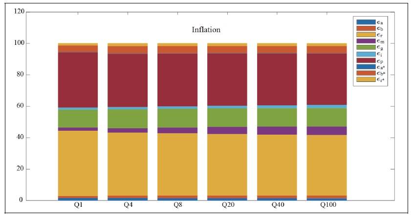
Finally, Figure 19 and Figure 20 present the decomposition of forecast error variances in output and inflation into components attributable to each of the model’s 10 orthogonal disturbances after the Asian Financial Crisis in the second subsample periods. Figure 19 shows that domestic markup and government spending shocks have mainly driven the variations in output after the crisis, which reflects the features of the Great Recession, as seen in Figure 15. Compared to the first subsample periods, it is noticeable the contribution of the government spending shock to the fluctuations of output has substantially increased in the second subsample periods. Figure 20 shows that monetary policy and risk premium shocks have dominated fluctuations in inflation, explaining approximately 60-80 percent of inflation at all horizons, as in the first subsample periods. It is noteworthy that the markup shock has also substantially contributed to fluctuations in inflation in the second subsample periods.
3)We assume that there is no constrained household in the large economy for the sake of analytical simplicity.
4)
IV. Concluding Remarks
This paper sets up a small, open economy, two-agent New Keynesian model and then investigates the role of constrained households in business cycles in Korea, employing a Bayesian estimation method. The paper finds that a large fraction of households in Korea were financially constrained before the Asian Financial Crisis. Still, this constraint has substantially increased after the crisis, as the traditional lifetime employment system collapsed and the Korean economy encountered the world-wide Great Recession.
Inspection of the driving forces of business cycles in Korea through the lens of the TANK model shows that domestic productivity, government spending, and markup shocks have dominated in explaining the behavior of output over business cycles in Korea since the mid-1970s. Still, domestic productivity has played a minor role in output variations after the Asian Financial Crisis with the prevalence of the world-wide Great Recession. The paper also finds that the risk premium shock has dominated both output and inflation fluctuations in Korea during the second subsample period, encompassing the world-wide Great Recession.
Tables & Figures
Table 1.
The Calibrated Parameters
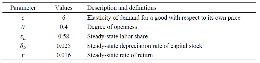
Table 2.
Bayesian Estimates of Key Parameters Before the Asian Financial Crisis (Sample Period: 1976:3Q - 1997:2Q)
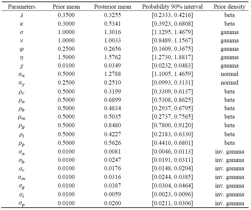
Table 3.
Bayesian Estimates of Key Parameters After the Asian Financial Crisis (Sample Period: 1998:3Q-2018:3Q)
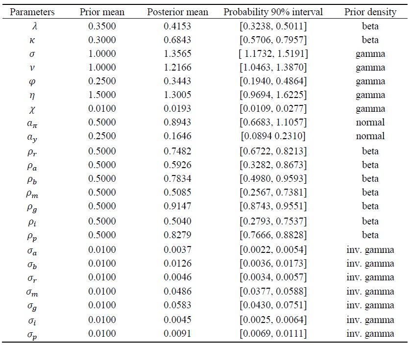
Figure 1.
Impulse Response to a Domestic Productivity Shock (Before the Asian Financial Crisis)
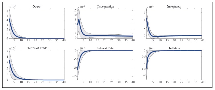
Figure 2.
Impulse Response to a Domestic Markup Shock (Before the Asian Financial Crisis)
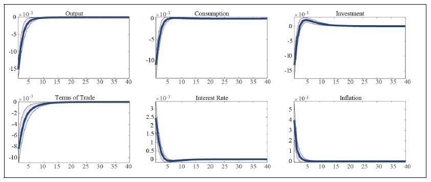
Figure 3.
Impulse Response to a Domestic Investment-Specific Productivity Shock (Before the Asian Financial Crisis)
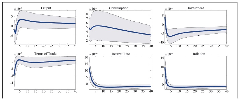
Figure 4.
Impulse Response to a Risk Premium Shock (Before the Asian Financial Crisis)
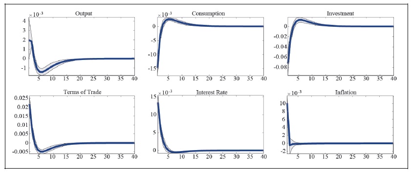
Figure 5.
Impulse Response to a Domestic Interest Rate Shock (Before the Asian Financial Crisis)
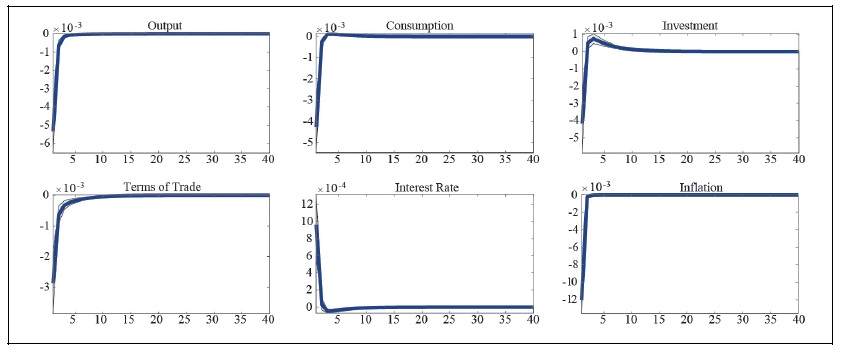
Figure 6.
Impulse Response to a Domestic Government Expenditure Shock (Before the Asian Financial Crisis)
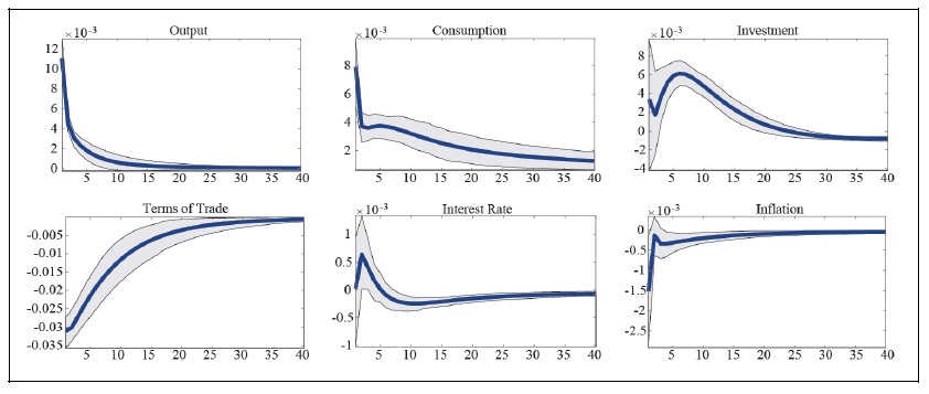
Figure 7.
Impulse Response to a Domestic Productivity Shock (After the Asian Financial Crisis)
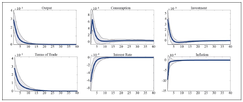
Figure 8.
Impulse Response to a Domestic Markup Shock (After the Asian Financial Crisis)
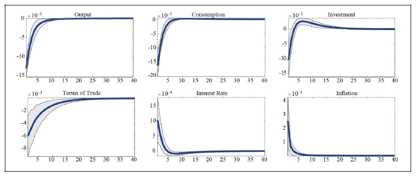
Figure 9.
Impulse Response to a Domestic Investment-Specific Productivity Shock (After the Asian Financial Crisis)
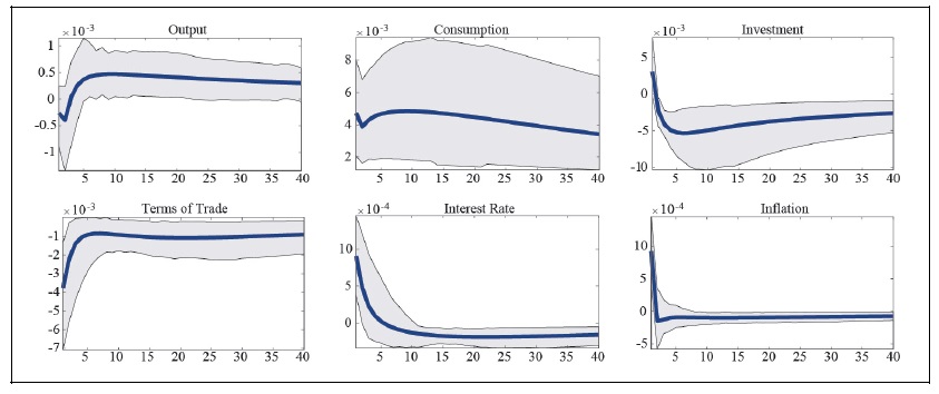
Figure 10.
Impulse Response to a Risk Premium Shock (After the Asian Financial Crisis)
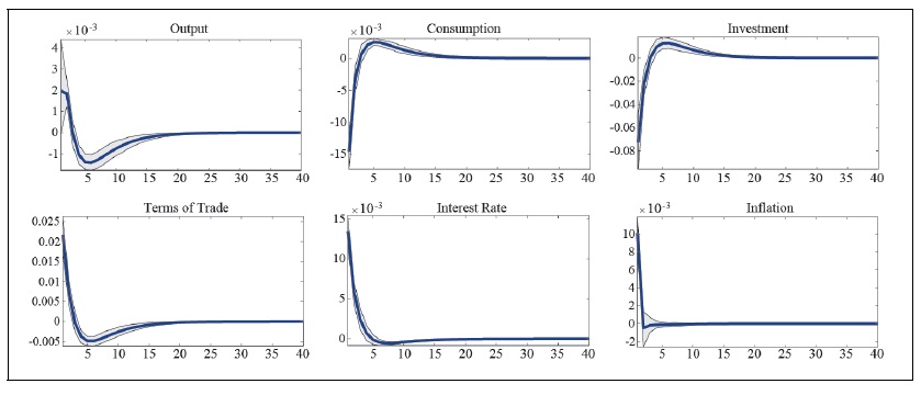
Figure 11.
Impulse Response to a Domestic Interest Rate Shock (After the Asian Financial Crisis)
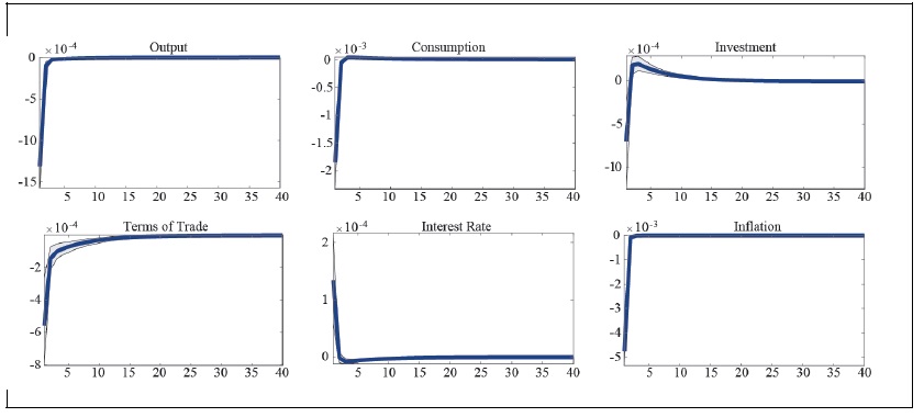
Figure 12.
Impulse Response to a Domestic Government Spending Shock (After the Asian Financial Crisis)
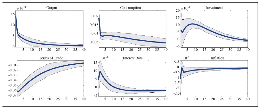
Figure 13.
Output Decomposition (Before the Asian Financial Crisis)
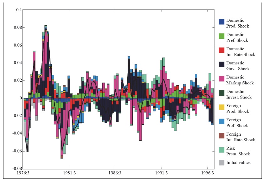
Figure 14.
Inflation Decomposition (Before the Asian Financial Crisis)
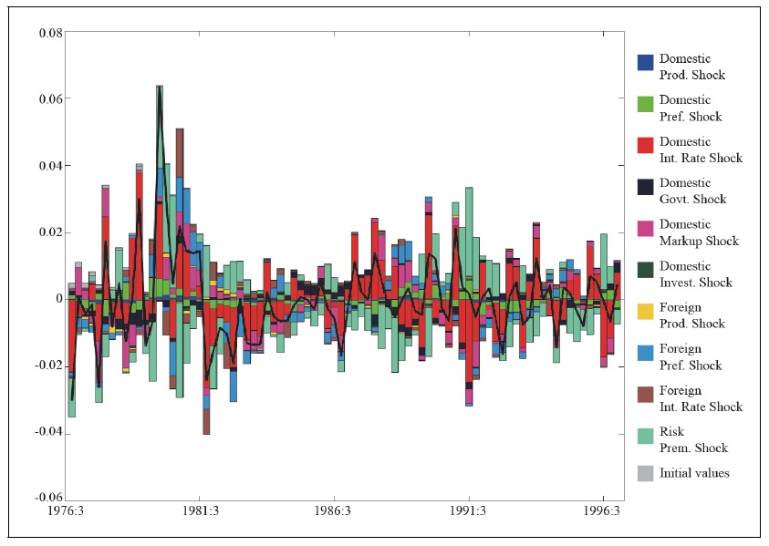
Figure 15.
Output Decomposition (After the Asian Financial Crisis)
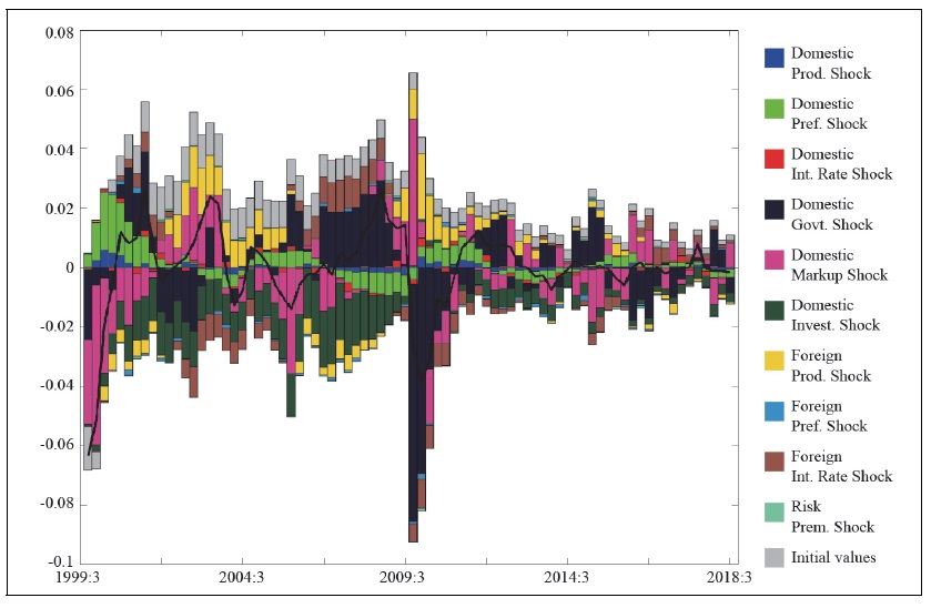
Figure 16.
Inflation Decomposition (After the Asian Financial Crisis)
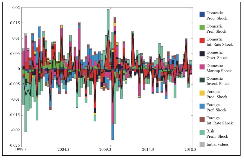
Figure 17.
Forecast Error Variance Decomposition (Before the Asian Financial Crisis)
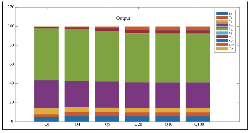
Figure 18.
Forecast Error Variance Decomposition (Before the Asian Financial Crisis)
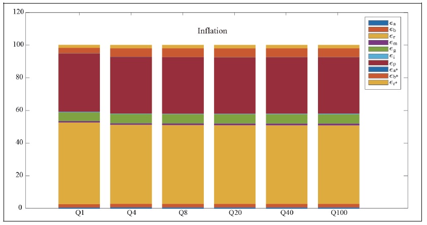
Figure 19.
Forecast Error Variance Decomposition (After the Asian Financial Crisis)
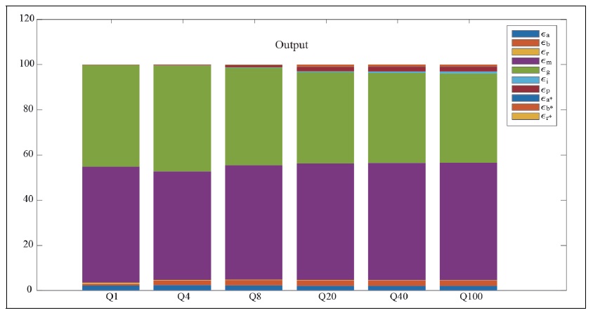
Figure 20.
Forecast Error Variance Decomposition (After the Asian Financial Crisis)
References
-
An, S.and F. Schorfheide. 2007. “Bayesian Analysis of DSGE Models.”
Econometric Reviews vol. 26, no. 2-4, pp. 113-172.
-
Auclert, A. 2019. “Monetary Policy and Redistribution.”
American Economic Review , vol. 109, no. 6, pp. 2333-2367.
-
Auclert, A., Rognlie, M. and L. Straub. 2024a. “The Intertemporal Keynesian Cross.”
Journal of Political Economy , vol. 132, no. 12.
-
Auclert, A., Rognlie, M. and L. Straub. 2024b. “Exchange Rates and Monetary Policy with Heterogeneous Agents: Sizing up and the Real Income Channel.” Stanford Univesity.
https://web.stanford.edu/~aauclert/ha_oe.pdf -
Bilbiie, F. O. 2008. “Limited Asset Market Participation, Monetary Policy, and (Inverted) Aggregate Demand Logic.”
Journal of Economic Theory , vol. 140, no. 1, pp.162-196.
-
Calvo, G. A. 1983. “Staggered Price in a Utility-maximizing framework.”
Journal of Monetary Economics , vol. 12, no, 3. pp. 383-398.
-
Dixit, A. K. and J. E. Stiglitz. 1977. “Monopolistic Competition and Optimum Product Diversity.”
American Economic Review , vol. 67, no. 3, pp. 297-308. -
Debortoli, D. and J. Gali. 2018. “Monetary Policy with Heterogeneous Agents: Insights from TANK Models.” CREI Working Paper.
http://www.crei.cat/wp-content/uploads/2018/03/dg_tank.pdf -
De Paoli, B. 2009. “Monetary Policy and Welfare in a Small Open Economy.”
Journal of International Economics , vol. 77, no. 1, pp. 11-22.
-
Faia, E. and T. Monacelli. 2008. “Optimal monetary policy in a small open economy with home bias.”
Journal of Money, Credit and Banking , vol. 40, no. 4, pp. 721-750.
-
Gali, J. and T. Monacelli. 2005. “Monetary Policy and Exchange Rate Volatility in a Small Open Economy.”
Review of Economic Studies , vol. 72, no. 3, pp. 707-734.
-
Gali, J., López-Saildo, J. D. and J. Vallés. 2007. “Understanding the Effects of Government Spending on Consumption.”
Journal of European Economic Association , vol. 5, no. 1, pp. 227-270.
-
Garcia-Cicco, J., Pancazi, R. and M. Uribe. 2010. “Real Business Cycles in Emerging Countries?,”
American Economic Review , vol. 100, no. 5, pp. 2510-2531.
-
Jung, Y. 2019. “What Drives Business Cycles in Korea?”
Japan and the World Economy , vol. 52.
-
Jung, Y. 2024. “Limited Financial Market Participations and Shocks in Business Cycles in Korea.”
East Asian Economic Review , vol. 28, no. 2, pp. 245-273.
-
Kaplan, G., Moll, B. and G. L. Violante. 2018. “Monetary Policy According to HANK.”
American Economic Review , vol. 108, no. 4, pp. 697-743.
-
Kulish, M. and D. Rees. 2011. “The Yield Curve in a Small Open Economy.”
Journal of International Economics , vol. 83, no. 2, pp. 268-279.
- Lee, S., Luetticke, R. and M. O. Ravn. 2023. “Shocks, Frictions, and Inequality in Korean Business Cycles.” BOK Working Paper, no. 2023-1.Bank of Korea.
-
Smets, F. and R. Wouters. 2007. “Shocks and Frictions in US Business Cycles: A Bayesian DSGE Approach.”
American Economic Review , vol. 97, no. 3, pp. 586-606.
-
Woodford, M. 2003.
Interest and Prices: Foundations of a Theory of Monetary Policy . Princeton, Princeton University Press. -
Yun, T. 1996. “Nominal price rigidity, money supply endogeneity, and business cycles.”
Journal of Monetary Economics , vol. 37, no. 2, pp.345-370.