

- EAER>
- Journal Archive>
- Contents>
- articleView
Contents
Citation
| No | Title |
|---|---|
| 1 | / 2020 / / vol.87, pp.84 / |
| 2 | What Determines Utility of International Currencies? / 2019 / Journal of Risk and Financial Management / vol.12, no.1, pp.10 / |
Article View
East Asian Economic Review Vol. 21, No. 4, 2017. pp. 317-342.
DOI https://dx.doi.org/10.11644/KIEP.EAER.2017.21.4.333
Number of citation : 2View
446
Download
278
Declining Japanese Yen in the Changing International Monetary System
|
|
Graduate School of Commerce and Management, Hitotsubashi University Research Institute of Economy, Trade and Industry |
|---|---|
|
|
Graduate School of Commerce and Management, Hitotsubashi University |

Abstract
The US dollar has kept as a position of key currency in the global economy in the changing international monetary system where the euro was introduced to some states of the EU in 1999. It is an evidence of inertia of the US dollar as a key currency. Our previous study (Ogawa and Muto, 2017b) conducted empirical analysis to investigate effects of several events on inertia of the US dollar. One of our findings was that the introduction of the euro increased utility of euro while utility of US dollar was kept unchanged. This paper examines the effects of the global financial crisis and the euro zone crisis as well as the introduction of the euro on the utility of the Japanese yen. The introduction of the euro significantly decreased the utility of the Japanese yen. It indicates that the introduction of the euro increased the utility of the euro while reducing the utility of the Japanese yen rather than the utility of the US dollar. The utility of the Japanese yen has significantly decreased while the global financial crisis and the euro zone crisis occurred. The Japanese yen has a declining trend in terms of its utility over time in the changing international monetary system.
JEL Classification: F33, F41, G01
Keywords
Japanese Yen, Utility of International Currency, Introduction of the Euro, Global Financial Crisis, Money-in-the-utility Function
I. INTRODUCTION
The international monetary system has been changing over time. Specifically, it is the introduction of the euro as a single common currency in 1999 that has changed it for the last several decades since the collapse of the Bretton Woods system. In the international monetary system, network externalities work in choosing a settlement currency. Utility of using an international currency for settlement depend on number of others who use it. Due to economies of scale related with the network externalities, there is inertia in a position of the US (United States) dollar as a key currency. In the situation, the euro which circulates in the large area of euro zone might have been a strong candidate against the US dollar.
However, the introduction of the euro has not significantly changed a position of the US dollar as a key currency due to its inertia in the current international monetary system. On one hand, the euro has become the second international currency in the world economy as well as a regional key currency in Europe.1 A possible consistent explanation for both the phenomena is that third international currencies such as the Japanese yen are declined in the international monetary system as a substitute for the euro. For the reason, this paper focuses on the Japanese yen as a third international currency to investigate whether the introduction of the euro has declined the Japanese yen in the international monetary system.
The Japanese yen is regarded as a third international currency in the international monetary system even though a share of the Japanese yen in euro-currency market is not so large. Ito, Koibuchi, Sato, and Shimizu (2013) conducted a questionnaire survey on the choice of invoicing currency with all Japanese manufacturing firms listed in the Tokyo Stock Exchange to show that the Japanese firms use the Japanese yen second to an importing country currency as invoice and trade settlement currencies in exporting products to the United States and Europe. On one hand, Japanese firms tend to use the Japanese yen as invoice and trade settlement currencies in exporting products to Asian countries. A share of Japanese yen-invoicing is larger than 50 percent for almost of destinations for Asian countries. Thus, the Japanese yen is one of the major international currencies especially in Asia.
In addition to the introduction of the euro, severe shortage of US dollar liquidity during the global financial crisis from August 2007 to December 2008 showed importance of the US dollar as a key currency in global financial markets. It is the current international monetary system with the US dollar as a key currency that is regarded as a background of the US dollar liquidity shortage in the global financial markets. The US dollar liquidity shortage had somewhat an adverse effect on usability or availability of the US dollar. Ogawa and Muto (2017b) conducted empirical analysis to show its negative effects on utility of the US dollar or specifically a parameter on the US dollar in the utility function according to money-in-the-utility model. In our previous study, we focused on effects of both the global financial crisis and the euro zone crisis on utility of the US dollar in order to clarify whether the US dollar has kept inertia as a key currency through the two crises.
This paper focuses on what happened against utility of the Japanese yen in the two crises and especially the US dollar liquidity shortage during the global financial crisis as well as after the introduction of the euro. We investigate whether the two crises as well as the introduction of the euro had any effects on utility of the Japanese yen. For our analysis, a money-in-the-utility model is used to take into account both functions as medium of exchange and as store of value of an international currency in the international currency competition. We estimate a parameter on an international currency in a utility function (afterwards we call it utility of an international currency) in the model. We base on the theoretical framework to conduct an empirical analysis regarding an issue whether the global financial crisis and the euro zone crisis as well as the introduction of the euro have changed utility of the Japanese yen.
In the next section, we explain our theoretical model, that is Sidrauski (1967)-type of money-in-the-utility model, according to Ogawa and Sasaki (1998) and Ogawa and Muto (2017b) in order to take into account both functions as medium of exchange and as store of value of international currencies. In the third section, we base on the theoretical model to conduct empirical analysis on whether utility of the Japanese yen changed after the global financial crisis and the euro zone crisis. In the fourth section, we summarize our empirical results and discuss a question to be solved in our future study.
1)
II. A THEORETICAL MODEL
We use the same theoretical model as that in Ogawa and Muto (2017b). It is based on a Sidrauski (1967)-type of money-in-the-utility model2 in which real balances of money as well as consumption are supposed as explanatory variables in a utility function. According to Ogawa and Sasaki (1998), we extend the money-in-the-utility model to one with parallel international currencies. A private sector maximizes a utility function in which real balances of international currencies as well as consumption depend on utility, subject to intertemporal budget constraint by taking into account an intertemporal fiscal budge constraint faced by a public sector.3
We focus on how the international currencies are held by private economic agents in a third country. For simplicity, we suppose that the monetary authorities of foreign major countries supply international currencies. The private sector in a third country holds international currencies as a result of their optimizing behavior. In other words, it has an optimal composition of international currencies to maximize utility.
For convenience, we suppose that it is the monetary authorities in both country
The monetary authorities in country
The private sector can save both liquidity costs4 and illiquidity costs5 by holding international currency
We suppose a situation that bonds in currencies
The private sector in country
Then, instantaneous budget constraints for the private sector are represented in real terms:


where  : real interest rate. Real interest rates in all countries are equal by both the uncovered interest parity and the purchasing power parity. A dot over variables means a change in the relevant variables.
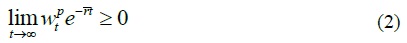
We assume no-Ponzi game conditions for the real balance of financial assets held by the private sector (
Equation (1a) can be rewritten as follows:

By taking into account a public sector with an intertemporal fiscal budge constraint  where
where

It is noteworthy that the real balance of currencies, that is, zero-interest liabilities, are included as negative terms in the budget constraint equation (1a’). The terms represent costs of holding currencies for the private sector. It reflects that the private sector has to pay seignorage to the relevant monetary authorities once it holds the currencies. The seignorage means inflation or depreciation of the relevant currencies and in turn lose the function as a store of value of the currencies.
We assume that the private sector maximizes its utility over an infinite horizon subject to budget constraints (1). We specify a Cobb-Douglas type of instantaneous utility function:
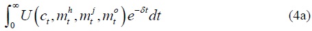
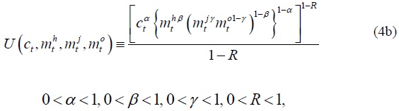
where
The private sector maximizes its utility functions (4a) and (4b) subject to budget constraint equation (3). We assume that the private sector has perfect foresight that economic variables do not diverge to infinity but converge to equilibrium values along a saddle path. The assumption rules out the possibility of multiplicity of equilibria in the model.
From the first-order conditions for maximization, an optimal share
where  : inflation rate of currency
  : inflation rate of currency
Equation (5) shows that the optimal share of international currency depends on both the inflation or depreciation rates of the international currencies and a parameter
Given parameter
2)
3)
4)The liquidity cost is an enactment cost in the
5)The illiquidity cost is a penalty cost of cash shortage in a precautionary demand for money model according to
III. EMPIRICAL ANALYSIS
1. Models for Estimating Utility of an International Currency
Here we suppose that international currencies include the US dollar, the euro, the Japanese yen, the Pound sterling, and the Swiss franc in order to analyze utility of the Japanese yen compared with the other four international currencies.6
We use equations (5) to estimate the parameters  The utility of international currency
  is transformed from equations (5) into the following equations:7
In this paper, we use equation (6a) to conduct empirical analysis of estimating utility of the Japanese yen by using data on 3-month or 6-month nominal interest rate. In addition, we use equation (6b) to conduct empirical analysis of estimating utility of the Japanese yen by setting 1.5%, 2.0%, 2.5%, or 3.0% as a real interest rate8.
We should use also a sum of the real interest rate and an expected inflation rate as a proxy of nominal interest rate because the nominal interest rate had strange movements especially during the global financial crisis when European financial institutes faced US dollar liquidity shortage. On the other hand, it is questionable whether it is adequate to use a sum of the real interest rate and an expected inflation rate as a proxy of nominal interest rate in a zero-bound interest rate period after the global financial crisis. For the reasons, we used both equation (6a) with a nominal interest rate and equation (6b) with a sum of the real interest rate and an expected inflation rate to conduct our empirical analysis.
2. Movements in Liquidity Risk Premium
We should look at movements in liquidity situation in international financial markets, especially interbank markets, during sample period before we set analytical periods. We use data on liquidity risk premium to identify liquidity situation.
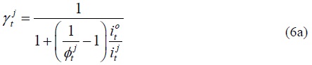
Figure 1a shows movements in three spreads of London Interbank Offered Rate (LIBOR) (US dollar, 3 months) minus US Treasury Bills (TB) rate (US dollar, 3 months), LIBOR (US dollar, 3 months) minus Overnight Indexed Swap (OIS) rate (US dollar, 3 months), and OIS rate (US dollar, 3 months) minus US TB rate (US dollar, 3 months). The spread of LIBOR minus OIS rate is regarded as credit risk premium because LIBOR is the interest rate at which banks borrow unsecured funds from other banks while OIS rate is the interest rate at which banks borrow secured funds from other banks. Given that banks mainly face credit risk and liquidity risk, the spread of OIS rate in terms of US dollar minus US TB rate is regarded as US dollar liquidity risk premium.
We can find that the credit risk premium had increased since August 2007 and explains most of movements in a spread between LIBOR and US TB rate in and after the Lehman Brothers bankruptcy in September 2008. On one hand, the US dollar liquidity risk premium had already increased since 2005. It approached its peak from August 2007 to September 2008. However, it has decreased to a level smaller than 0.1% since the Federal Reserve Board (FRB) started quantitative easing monetary policy late 2008 when it at the same time concluded and extended currency swap arrangements9 with other major central banks to provide US dollar liquidity to other countries.
Figure 1b show movements in the three spreads in international financial markets in terms of the Japanese yen. It had different characteristics compared with that of the US dollar. We cannot find that liquidity risk premium for the Japanese yen had no increase during the period from 2007 to 2008. The stable movements in the liquidity risk premium for the Japanese yen is different those for the US dollar. The reason is that the global financial crisis had little adverse effect on Japanese financial markets.
3. Analytical Periods
A whole sample period covers a period from 1986Q1 to 2016Q210 due to data availability. We divide the whole sample period into several sub-sample periods to analyze whether the global financial crisis and the euro zone crisis as well as the introduction of the euro changes utility of international currencies on January 1, 1999.
Figure 1a shows that financial institutions in Europe had faced US dollar liquidity shortage since the BNP Paribas shock happened in August 2007. We investigate whether the global financial crisis, especially the BNP Paribas shock in 2007Q3 had any effects on utility of the US dollar. We divide the whole sample period into three sub-sample periods which include a period from 1986Q1 to 1998Q4, a period from 1999Q1 to 2007Q2, and a period from 2007Q3 to 2016Q2. We analyze differences in utility of international currencies between sub-sample periods 1986Q1-1998Q4 and 1999Q1-2007Q2 to investigate effects of the introduction of euro on utility of international currencies. Moreover, we analyze differences in utility of international currencies between sub-sample periods 1999Q1-2007Q2 and 2007Q3-2016Q2 to investigate effects of the BNP Paribas shock on utility of international currencies. Financial institutions faced the US dollar liquidity shortage during the sub-sample period 2007Q3-2016Q2.
Next, we investigate whether the global financial crisis, especially the bankruptcy of Lehman Brothers in September 2008 had any effects on utility of international currencies. We divide the whole sample period into three sub-sample periods which include a period from 1986Q1 to 1998Q4, a period from 1999Q1 to 2008Q2, and a period from 2008Q3 to 2016Q2. We analyze differences in utility of international currencies between sub-sample periods 1999Q1-2008Q2 and 2008 Q3-2016Q2 to investigate effects of the Lehman shock on utility of international currencies. Financial institutions faced the US dollar liquidity risk as well as credit risk during the sub-sample period 2008Q3-2016Q2.
Moreover, we investigate whether the euro zone crisis had any effects on utility of international currencies. The euro zone crisis started once the Greek debt crisis occurred late in 2009. We divide the whole sample period into three sub-sample periods which include a period from 1986Q1 to 1998Q4, a period from 1999Q1 to 2009Q3, and a period from 2009Q4 to 2016Q2. We analyze differences in utility of international currencies between sub-sample periods 1999Q1-2009Q3 and 2009Q4-2016Q2 to investigate effects of the euro zone crisis on utility of the international currencies.
4. Data
The shares of the US dollar, the euro, the Japanese yen, the Pound sterling, and the Swiss franc are calculated according to the theoretical model in which we regard that the real balances of international currencies contribute to utility. However, it is difficult to obtain data on the real balance of international currency held by private sector in the world economy. Instead, we use BIS data on total of domestic currency denominated debt and foreign currency denominated debt of the euro currency market according to the previous study (Ogawa and Sasaki, 1998; Ogawa and Kawasaki, 2001). Specifically, we use total data of domestic currency denominated debts and foreign currency denominated debts in the euro currency markets as nominal balances of the relevant currency or a numerator of  The data are obtained from a website of Bank for International Settlements (BIS). Given a data constraint that the data are quarterly, we have to use quarterly data of other variables to conduct the empirical analysis.
100% stacked area charts of total of domestic currency denominated debt and foreign currency denominated debt of the euro currency market are shown in Figures 2. Figure 2 shows movements in shares of foreign currency denominated debt of the euro currency market classified by currencies. The share of the US dollar has decreased while the share of the euro has increased in 1998Q4. The decreases in the share of the euro occurred because euro zone currencies have replaced the euro by the introduction of the euro. In other words, euro zone residents increased domestic currency (the euro) and decrease foreign currency (the euro zone currencies except home currencies). Figure 2b shows movements in shares of all currency denominated debt of the euro currency market classified by currencies. In this figure, the share of the euro has increased little by little because the above effects were canceled out.
We use 3-month LIBOR and 6-month LIBOR data as the nominal interest rate. The data are obtained from a website of International Financial Statistics (IMF).  is a weighted average of nominal interest rates in terms of the four other currencies. The weights are based on outstanding of foreign currency denominated debts. Data on the euro denominated nominal interest rate are not available from 1986Q1 to 1998Q4. Instead, we use an arithmetical average the LIBOR in terms of the French franc, the Deutsche Mark and the Netherland Guilder. The data are obtained from a website of IMF.
Expected inflation rates are calculated from current price level and expected price level. We assume that the price level of each period follows ARIMA (p, d, q) process. Secondly, we use monthly data on the price level for the last twenty-eight years to estimate an ARIMA model. The BIC is used for lag selection. Thirdly, the estimated ARIMA model is used to predict a price level of one period ahead. Finally, we use the actual price level and the predicted price level of one period ahead to calculate the expected inflation rate. Consumer price index data are used as the price level. The data are obtained from a website of Organisation for Economic Co-operation and Development (OECD).
The expected inflation rate in the euro zone is a weighted average of the expected inflation rate in the original euro zone countries. They include Austria, Belgium, Finland, France, Germany, Ireland, Italy, Luxembourg, Netherlands, Portugal, and Spain. A weight in calculating a weighted average of the expected inflation rate is based on GDP share among the countries. The data obtained from Penn World Table website.11
5. Analytical Method
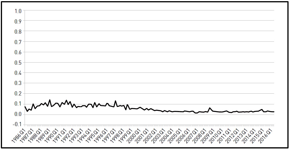
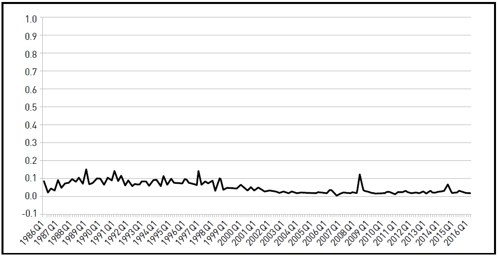
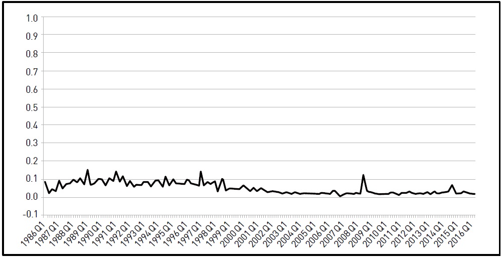
We conduct point estimation for utility of the Japanese yen in each quarter during a sample period from 1986Q1 to 2016Q2. We exclude results of point estimation which are regarded as outliers because they exceed plus/minus three times of standard deviation from its estimation. Time series of utility of the Japanese yen are shown in Figures 3a to 3f. Based on the point estimation, we calculate a mean value of the contribution in each of the sub-sample periods. We compare the mean values among the sub-sample periods to investigate whether the utility of the currency statistically significantly increased or decreased. For the purpose, we use the Welch’s t test to test difference in the mean values among the sub-sample periods.
The Welch’s t test is used to test whether the population mean of the two samples is the same. Hypothesis is as follows:
If the null hypothesis
6. Analytical Results
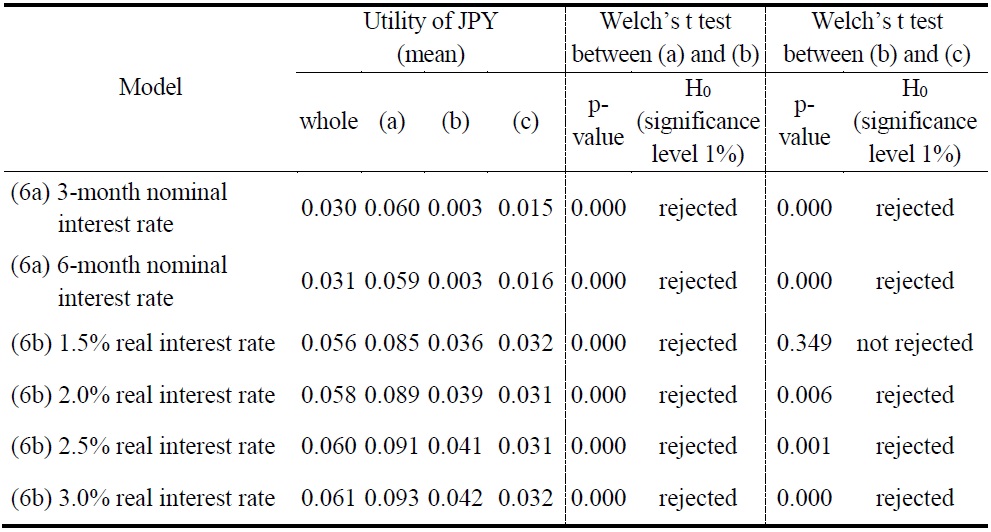
Table 1 shows analytical results of the utility of the Japanese yen in the sub-sample periods 1986Q1-1998Q4, 1999Q1-2007Q2, and 2007Q3-2016Q2 by focusing on effects of the introduction of the euro and the BNP Paribas shock on the utility of the Japanese yen. In Table 1a, the first row shows which model is used for estimation of utility of the Japanese yen. The first line shows analytical results in the case of using data on 3-month nominal interest rate in the model (6a). The second line shows analytical results in the case of using data on 6-month nominal interest rate in the model (6a). The third line shows analytical results in the case of setting 1.5% as a real interest rate in the model (6b). The fourth line shows analytical results in the case of setting 2.0% as a real interest rate in the model (6b). The fifth line shows analytical results in the case of setting 2.5% as a real interest rate in the model (6b). The sixth line shows analytical results in the case of setting 3.0% as a real interest rate in the model (6b).
Rows of “Utility of JPY (mean)” show means of the utility of the Japanese yen in each of whole sample period and sub-sample periods. Column (a) shows means of the utility of the Japanese yen before the introduction of euro. Means of the utility of the Japanese yen is 0.059-0.093 before the introduction of euro. Column (b) shows means of the utility of the Japanese yen after the introduction of euro and before the BNP Paribas shock. Means of the utility of the Japanese yen after the introduction of euro are 0.002-0.043. Column (c) shows means of the utility of the Japanese yen after the BNP Paribas shock. Column (c) shows that the utility of the Japanese yen is 0.015-0.032 after the BNP Paribas shock.
Columns of “Welch’s t test between (a) and (b)” and “Welch’s t test between (b) and (c)” show p-values of the Welch’s t test and rejection of the hypothesis that means significantly equal between sub-sample periods 1986Q1-1998Q4 and 1999Q1-2007Q2, and between sub-sample periods 1999Q1-2007Q2 and 2007Q3-2016Q2 at the 1% level, respectively. The results of the Welch’s t test between sub-sample periods 1986Q1-1998Q4 and 1999Q1-2007Q2 show that the hypothesis of equal means between sub-sample periods 1986Q1-1998Q4 and 1999Q1-2007Q2 is rejected at all of the models. It implies that the utility of the Japanese yen decreased before and after the introduction of the euro.
The results of the Welch’s t test between sub-sample periods 1999Q1-2007Q2 and 2007Q3-2016Q2 show that the hypothesis of equal means between sub-sample periods 1999Q1-2007Q2 and 2007Q3-2016Q2 is rejected in all of the models except for in the case of setting 1.5% real interest rate in the model (6b). The utility of the Japanese yen has made statistically significant decreased before and after the BNP Paribas shock in the model (6b) except for the case of setting 1.5% real interest rate. The utility of the Japanese yen has decreased to 0.031. On the other hand, the utility of the Japanese yen has made statistically significant increased before and after the BNP Paribas shock in the model (6a). However, it has decreased from 0.059-0.060 in the sub-sample period 1986Q1-1998Q4 to 0.015-0.016 in the sub-sample period 2007Q3-2016Q2. It is clear that it has a declining trend in the long run.
Table 2 shows analytical results of the utility of the Japanese yen in the sub-sample periods 1986Q1-1998Q4, 1999Q1-2008Q2, and 2008Q3-2016Q2 by focusing on effects of the Lehman Brothers bankruptcy on the utility of the euro. The utility of the Japanese yen is 0.059-0.093 before the introduction of the euro. The utility of the Japanese yen is 0.003-0.042 before the Lehman Brothers bankruptcy and after the introduction of euro. The results of the Welch’s t test between sub-sample periods 1986Q1-1998Q4 and 1999Q1-2008Q2 show that the hypothesis of equal means between sub-sample periods 1986Q1-1998Q4 and 1999Q1-2008Q2 is rejected in all of the models. It implies that the introduction of the euro decreased the utility of the Japanese yen before the Lehman Brothers bankruptcy.
The utility of the Japanese yen is 0.015-0.032 after the Lehman Brothers bankruptcy. The results of the Welch’s t test between sub-sample periods 1999Q1-2008Q2 and 2008Q3-2016Q2 show that the hypothesis of equal means between sub-sample periods 1999Q1-2008Q2 and 2008Q3-2016Q2 is rejected in all of the models except for the cases of setting 1.5% as a real interest rate in the model (6b). The utility of the Japanese yen has made statistically significant decreased before and after the Lehman Brothers bankruptcy in the model (6b) except for the case of setting 1.5% real interest rate. The utility of the Japanese yen has decreased to 0.031. On the other hand, the utility of the Japanese yen has made statistically significant increased before and after the Lehman Brothers bankruptcy in the model (6a). It has increased to 0.015-0.016. However, it has decreased from 0.059-0.060 in the sub-sample period 1986Q1-1998Q4 to 0.015-0.016 in the sub-sample period 2008Q3-2016Q2. It is clear that the Japanese yen has a declining trend in the long run.
Table 3 shows analytical results of the utility of the Japanese yen in the sub-sample periods 1986Q1-1998Q4, 1999Q1-2009Q3, and 2009Q4-2016Q2 by focusing on effects of the Greek debt crisis on the utility of the euro. The utility of the Japanese yen is 0.059-0.093 before the introduction of the euro. The utility of the Japanese yen is 0.005-0.042 before the Greek debt crisis and after the introduction of the euro. The results of the Welch’s t test between sub-sample periods 1986Q1-1998Q4 and 1999Q1-2009Q3 show that the hypothesis of equal means between sub-sample periods 1986Q1-1998Q4 and 1999Q1-2009Q3 is rejected at all of the models. The introduction of the euro decreased the utility of the Japanese yen before the Greek debt crisis.
The utility of the Japanese yen is 0.015-0.030 after the Greek debt crisis. The results of Welch’s t test between sub-sample periods 1999Q1-2009Q3 and 2009Q4-2016Q2 show that the hypothesis of equal means between sub-sample periods 1999Q1-2009Q3 and 2009Q4-2016Q2 is rejected at all the models except for the case of setting 1.5% as a real interest rate in the model (6b). It implies that the utility of the Japanese yen has changed before and after the Greek debt crisis though the hypothesis is not rejected in the one case. However, movements in the utility of the Japanese yen significantly increased before and after the Greek debt crisis in the models (6a) were regarded to be abnormal because those were 0.005 in the sub-sample period 1999Q1-2009Q3. On the other hand, in the cases of using real interest rate data, the utility of the Japanese yen decreased from 0.039-0.042 during a period from the introduction of the euro to two crises to 0.029-0.030 through the two crises.
In summary, it is clear that the introduction of the euro decreased the utility of the Japanese yen. The decrease in the utility of the Japanese yen can explain the finding in Ogawa and Muto (2017b) that the introduction of the euro increased the utility of the euro while the utility of the US dollar was unchanged. Moreover, Ogawa and Muto (2017a) found that the utility of the Swiss franc as well decreased after the introduction of the euro. It seems that it is not the US dollar but the Japanese yen and the Swiss franc that substitute for the euro in the international monetary system.
Moreover, we obtained that the BNP Paribas shock, the Lehman Brothers bankruptcy, and the Greek debt crisis significantly changed the utility of the Japanese yen in five of all six cases. Especially when we use real interest rates and expected inflation instead of nominal interest rates, the utility of the Japanese yen significantly decreased after the BNP Paribas shock, the Lehman Brothers bankruptcy, and the Greek debt crisis occurred. Given that it significantly decreased after the introduction of the euro, it seems that the Japanese yen has a decreasing trend in terms of its utility over the global financial crisis and the euro zone crisis. Also in the long run, comparison in utility of the Japanese yen between pre-introduction of the euro and both of the crises show a declining trend of utility of the Japanese yen.
6)
7)We suppose that parameter  might change over time because we have an important objective to investigate how the parameter changed during the analytical period though it seems to be stable as a deep parameter.
8)
9)The FRB concluded new currency swap arrangements with the European Central Bank (ECB) and the Swiss National Bank on December 12, 2007. Afterwards, it increased amount of currency swap arrangements and concluded them with other central banks.
10)In
11)See
IV. CONCLUSION
In this paper, we based on a theoretical background of a money-in-the-utility model to investigate utility of the Japanese yen as an international currency while we suppose the other international currencies which include the US dollar, the euro, the Pound sterling, and the Swiss franc. Specifically, we estimated effects of the global financial crisis and the euro zone crisis as well as the introduction of the euro on utility of the Japanese yen.
The utility of the Japanese yen has significantly decreased after the introduction of euro. This corresponds to the increase in utility of the euro while the utility of the US dollar had unchanged after the introduction of the euro. The introduction of the euro has enhanced the utility of the euro by substituting it for not the US dollar but the Japanese yen. It is evidence that the US dollar has inertia as a key currency in the current international monetary system. Ogawa and Muto (2017a) found that the utility of the Swiss franc also decreased at the same time when the utility of the Japanese yen decreased after the introduction of the euro. It implies that the Japanese yen as well as the Swiss franc are substitute for the euro.
Moreover, the BNP Paribas shock, the Lehman Brothers bankruptcy, and the Greek debt crisis significantly decreased the utility of the Japanese yen when we use sum of real interest rates and expected inflation rate instead of nominal interest rates. It seems that the Japanese yen has a declining trend in terms of its utility over time after the introduction of euro and then through the global financial crisis and the euro zone crisis.
We should consider why the Japanese yen has a declining trend in terms of its utility over time after the introduction of euro and then through the global financial crisis and the euro zone crisis. One of the backgrounds might be related with decreasing Japanese share of GDP and international trade in the global economy while the Japanese economy has experienced “lost two decades”. We should conduct an empirical analysis to investigate what factors decline the utility of the Japanese yen as an international currency. The question is to be solved in our future study.
Tables & Figures
Figure 1a.
Credit Risk Premium and Liquidity Risk Premium for the USD
Data: Datastream, Credit risk = London Interbank Offered Rate (LIBOR) (USD, 3 months) minus Overnight Indexed Swap (OIS) rate (USD, 3 months), liquidity risk = OIS minus US Treasury Bills (TB) rate (USD, 3 months)
Figure 1b.
Credit Risk Premium and Liquidity Risk Premium for the JPY
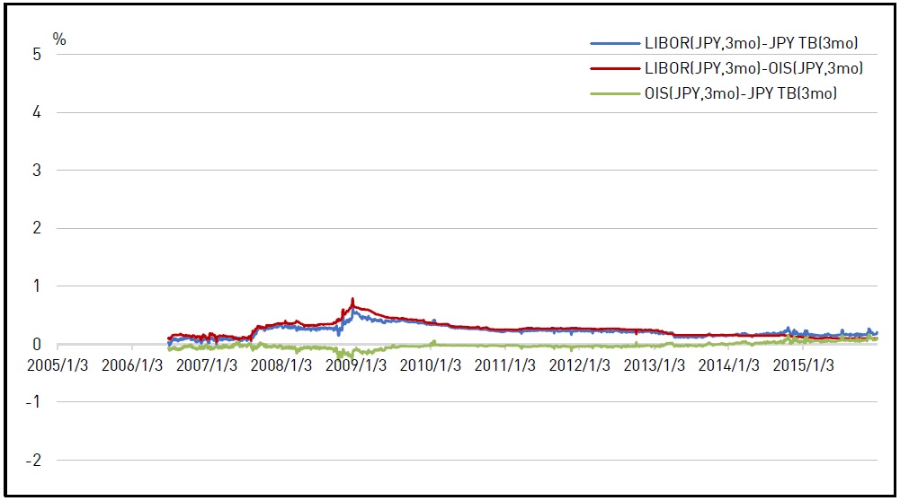
Data: Datastream, Credit risk = London Interbank Offered Rate (LIBOR) (JPY, 3 months) minus Overnight Indexed Swap (OIS) rate (JPY, 3 months), liquidity risk = OIS minus yields on Japanese Treasury Discount Bills (JPY TB rate) (JPY, 3 months)
Figure 2.
All Currency Denominated Debt of the Euro Currency Market
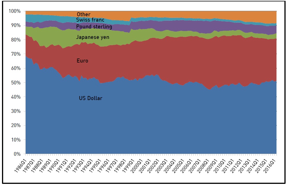
Data: BIS
Figure 3a.
Utility of the JPY in the Case of Using Data on 3-month Nominal Interest Rate in Model (6a)
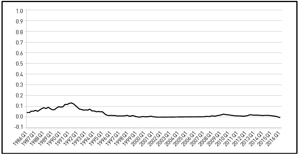
*Outliers which are beyond three times of standard deviation are excluded from our sample.
Figure 3b.
Utility of the JPY in the Case of Using Data on 6-month Nominal Interest Rate in Model (6a)
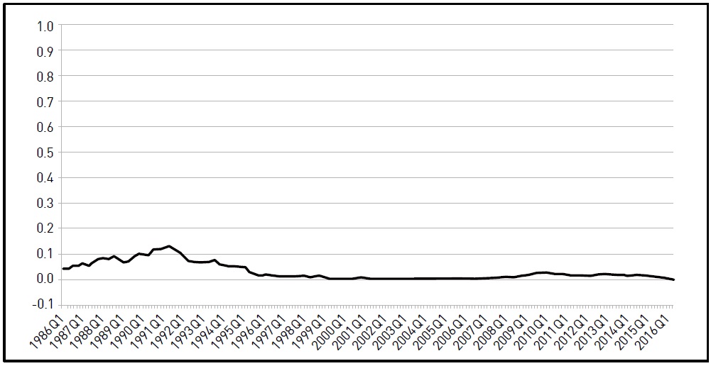
*Outliers which are beyond three times of standard deviation are excluded from our sample.
Figure 3c.
Utility of the JPY in the Case of Setting 1.5% as a Real Interest Rate in Model (6b)

*Outliers which are beyond three times of standard deviation are excluded from our sample.
Figure 3d.
Utility of the JPY in the Case of Setting 2.0% as a Real Interest Rate in Model (6b)
*Outliers which are beyond three times of standard deviation are excluded from our sample.
Figure 3e.
Utility of the JPY in the Case of Setting 2.5% as a Real Interest Rate in Model (6b)
*Outliers which are beyond three times of standard deviation are excluded from our sample.
Figure 3f.
Utility of the JPY in the Case of Setting 3.0% as a Real Interest Rate in Model (6b)
*Outliers which are beyond three times of standard deviation are excluded from our sample.
Table 1.
Utility of the JPY in the Sub-sample Periods Devided the Introduction of the Euro and BNP Paribas Shock
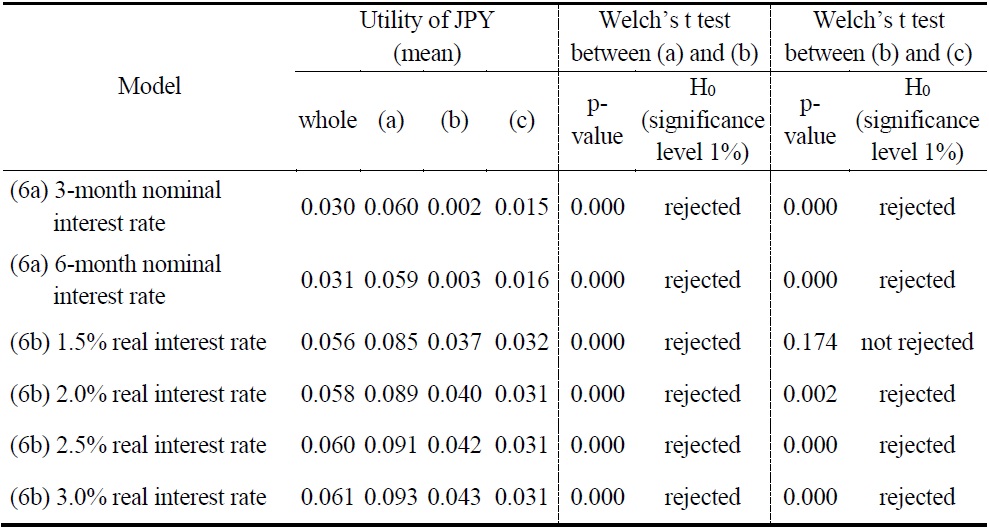
*whole:1986Q1-2016Q2, (a):1986Q1-1998Q4, (b):1999Q1-2007Q2, (c):2007Q3-2016Q2
Table 2.
Utility of the JPY in the Sub-sample Periods Devided the Introduction of the Euro and Lehman Brothers Bankruptchy
* whole:1986Q1-2016Q2, (a):1986Q1-1998Q4, (b):1999Q1-2008Q2, (c):2008Q3-2016Q2
Table 3.
Utility of the JPY in the Sub-sample Periods Devided the Introduction of the Euro and Greek Debt Crisis
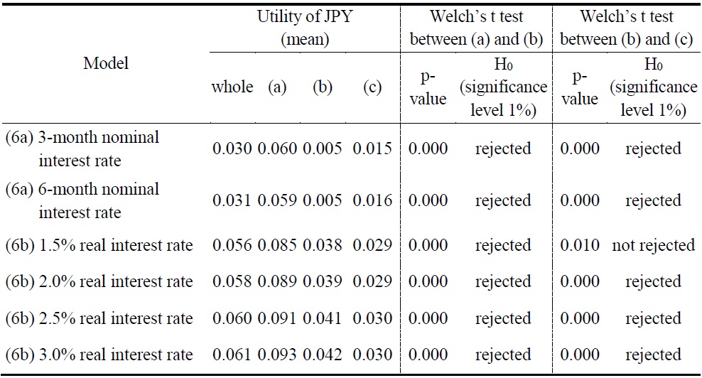
*whole:1986Q1-2016Q2, (a):1986Q1-1998Q4, (b):1999Q1-2009Q3, (c):2009Q4-2016Q2
References
-
Baumol, W. J. 1952. “The Transactions Demand for Cash: An Inventory Theoretic Approach,”
Quarterly Journal of Economics , vol. 66, no. 4, pp. 545-556.
-
Blanchard, O. J. and S. Fischer. 1989.
Lectures on Macroeconomics . Cambridge, MA: MIT Press. -
Calvo, G. A. 1981. “Devaluation: Level Versus Rates,”
Journal of International Economics , vol. 11, no. 2, pp. 165-172.
-
Calvo, G. A. 1985. “Currency Substitution and the Real Exchange Rate: The Utility Maximization Approach,”
Journal of International Money and Finance , vol. 4, no. 2, pp. 175-188.
-
European Central Bank (ECB). 2017.
The International Role of the Euro . Frankfurt, Germany. -
Feenstra, R. C., Inklaar R. and M. P. Timmer. 2015. “The Next Generation of the Penn World Table,”
American Economic Review , vol. 105, no. 10, pp. 3150-3182.
- Ito, T., Koibuchi, S., Sato, K. and J. Shimizu. 2013. Choice of Invoicing Currency: New Evidence from a Questionnaire Survey of Japanese Export Firms. RIETI Discussion Paper Series, no. 13-E-034.
-
Matsuyama, K., Kiyotaki, N. and A. Matsui. 1993. “Toward a Theory of International Currency,”
Review of Economic Studies , vol. 60, no. 2, pp. 283-307.
-
Obstfeld, M. 1981. “Macroeconomic Policy, Exchange-rate Dynamics, and Optimal Asset Accumulation,”
Journal of Political Economy , vol. 89, no. 6, pp. 1142-1161.
- Ogawa, E. and K. Kawasaki, 2001. Effects of the Introduction of the Euro on International Monetary System. Hitotsubashi University Graduate School of Commerce and Management Discussion Paper, no. 63. (in Japanese)
- Ogawa, E. and M. Muto. 2017a. Declining Japanese Yen and Inertia of the U.S. Dollar. RIETI Discussion Paper Series, no. 17-E-018.
-
Ogawa, E. and M. Muto. 2017b. “Inertia of the U.S. Dollar as a Key Currency Through the Two Crises,”
Emerging Markets Finance and Trade , vol. 53, no. 12, pp. 2706-2724.
-
Ogawa E. and Y. N. Sasaki. 1998. “Inertia in the Key Currency,”
Japan and the World Economy , vol. 10, no. 4, pp. 421-439.
-
Tobin, J. 1956. “The Interest Elasticity of Transaction Demand for Cash,”
Review of Economics and Statistics , vol. 38, no. 3, pp. 241-247.
-
Trejos, A. and R. Wright. 1996. “Search-Theoretic Models of International Currency,”
Review , Federal Reserve Bank of St. Louis, vol. 78, no. 3, pp. 117-132. -
Weil, P. 1991. Currency Competition and the Transition to Monetary Union: Currency Competition and the Evolution of Multi-currency Regions. In Giovannini, A. and C. Mayer. (eds.)
European Financial Integration . Cambridge: Cambridge University Press. pp. 290-304. -
Welch, B. L. 1938. “The Significance of the Difference Between Two Means When the Population Variances are Unequal,”
Biometrika , vol. 29, no. 3/4, pp. 350-362.
-
Whalen, E. L. 1966. “A Rationalization of the Precautionary Demand for Cash,”
Quarterly Journal of Economics , vol. 80, no. 2, pp. 314-324.
-
Woodford, M. 1991. Currency Competition and the Transition to Monetary Union: Does Competition Between Currencies Lead to Price Level and Exchange Stability?,” In Giovannini, A. and C. Mayer. (eds.)
European Financial Integration . Cambridge: Cambridge University Press. pp. 257-289.