

- EAER>
- Journal Archive>
- Contents>
- articleView
Contents
Citation
Article View
East Asian Economic Review Vol. 25, No. 1, 2021. pp. 33-71.
DOI https://dx.doi.org/10.11644/KIEP.EAER.2021.25.1.390
Number of citation : 7View
98
Download
109
Non-Tariff Trade Policy in the Context of Deep Trade Integration: An Ex-Post Gravity Model Application to the EU-South Korea Agreement
|
|
Vienna Institute for International Economic Studies |
|---|---|
|
|
Vienna Institute for International Economic Studies |

Abstract
Many different approaches and databases have been developed for the evaluation of non-tariff measures (NTMs) and free trade agreements (FTAs). This paper is devoted to the EU-South Korea agreement, which is the first ‘second-generation’ FTA of the EU, addressing a wide array of non-tariff policies. We review the evolution of NTM types applicable to the EU-South Korea trade relationship and the role of NTMs in ex-ante and ex-post analyses of the agreement. Subsequently a structural gravity model is employed to assess the value added of information on different aspects of FTAs and types of NTMs by evaluating their ability to predict the trade effects of the EU-South Korea FTA. Our results show that, when accounting for information on the components common in modern deep trade agreements, no additional trade effect is attributable to the EU-South Korea FTA. The evolution of NTMs differs considerably across indicators used, but trade predictions are hardly affected. Most specifications point towards a negative effect of bilateral differences in the number of technical barriers to trade (TBT) applied and sanitary and phytosanitary measures (SPS) against which trading partners issued complaints at the WTO.
JEL Classification: C54, F13, F14
Keywords
Trade Policy, Free Trade Agreement, EU, South Korea, Gravity Model
I. Introduction: Time is Ripe for Ex-Post Estimations using NTMs
The importance of tariffs as a trade policy tool for international trade in nonagricultural goods has diminished since the establishment of the General Agreement on Tariffs and Trade (GATT) in 1948. However, non-tariff measures (NTMs) and free trade agreements (FTAs) regulating trade issues beyond tariff cuts have been on the rise since the mid-1990s. Although tariff data and trade data are abundant, data work on NTMs is still in its infancy. Research on the economic implications of NTMs is evolving, as are different data collection methods, measurement and estimation procedures.
This paper aims to shed light on how information on NTMs can be best used for empirical analysis. To do so, we model NTMs for the analysis of trade flows between the European Union (EU) and South Korea (KR) in a structural gravity setting and evaluate multiple indicators of NTMs based on their ability of predicting trade flows by performing an ex-post estimation.
South Korea is chosen because it is the first trading partner with which the EU has established a deep and comprehensive second-generation FTA, reaching far beyond tariff cuts. As such, it is the first EU trade agreement, where the analysis of NTMs is a relevant research topic. It was provisionally applied from mid-2011 and entered fully into force in December 2015. However, it was not the last economy in Asia with which the EU has negotiated deep agreements. The EU-Japan Economic Partnership Agreement (EPA) entered into force on 1 February 2019, the FTA with Singapore on 21 November 2019 and the FTA with Vietnam on 1 August 2020. Negotiations with other countries – partly to modernise existing agreements – are ongoing.
Although several ex-ante studies on the EU-KR agreement were conducted, ex-post evaluations are still scarce. In view of the revival of bilateral and plurilateral FTA negotiations, partly accelerated by growing trade tensions between China and the US, it is worth reviewing strategies for the evaluation of the ‘role model’ of today’s FTA negotiations.
The paper is structured as follows. The reminder of section I describes different ways in which NTMs enter econometric analysis in the literature and illustrates what these measures look like if applied to a comprehensive NTM dataset (WTO I-TIP). Section II briefly reviews the EU-KR FTA, and describes the structural gravity model and the data used to perform the ex-post estimation. Section III presents empirical results and section IV provides our conclusions.
1. NTMs in Different Shapes
When policy makers communicate (expected) gains from trade deals to the public, they primarily refer to tariffs. Tariffs are relatively easy to understand and the effects of tariff cuts seem rather obvious: ideally, when duties fall, trading becomes cheaper, prices for companies and consumers should fall, and trade volumes should rise. The forms of NTMs – ranging from standard-like regulations, through temporary trade defence measures to special trade instruments for the protection of the agricultural sector – are diverse and their impact ambiguous as they often affect multiple spheres and may represent different consumer preferences. NTMs still constitute ‘
The perception of NTMs as murky trade policy instruments (Evenett, 2019) might well change with the efforts undertaken to make their application more transparent and measurable. Until recently, economists have often had to set up their own product- and country-specific NTM datasets for work on their research questions.1 However, extensive datasets covering a wide range of products and countries are emerging. The first of its kind was developed for antidumping measures (Bown, 2005). Since 2006, international organisations have been joining forces in a Multi-Agency Support Team (MAST)2 to improve the classification, collection and use of information on NTMs for academics and policy makers. Since then, data on antidumping activities have been complemented by more types of contingent protection measures by the World Bank (Bown, 2016). Joint efforts by international institutions have also led to a database of indices for several NTM types (Gourdon, 2014), provided by CEPII.
To the best of our knowledge, there are three truly comprehensive datasets covering a wide range of countries and NTM types.3 UNCTAD’s Trade Analysis Information System (TRAINS) and the Global Trade Alert (GTA) by CEPR have collected information, primarily from official sources, since the onset of the global economic and financial crisis in 2008. The third dataset is the WTO’s Integrated Trade Intelligence Portal (I-TIP), which covers publicly available information on notifications of NTMs to the WTO since its establishment, as well as complaints raised against trading partners in the form of specific trade concerns (STCs). We make use of the wiiw NTM Data: in this, data from the WTO I-TIP has been complemented by non-duplicate NTMs in the Temporary Trade Barriers Database (TTBD) compiled by Bown (2016) and enhanced by imputing missing 6-digit product codes of the Harmonised System (HS) (Grübler and Reiter, 2020).4 We are aware that notifications data tend to suffer from notification biases (Bacchetta et al., 2012), in particular for smaller and less developed economies. However, the data have compensatory advantages: they reach back to 1995 and provide detailed accounts for so-called standard-like NTMs, i.e. sanitary and phytosanitary measures (SPS) and technical barriers to trade (TBTs), which feature prominently in the EU’s second-generation FTAs.
In addition to different NTM data collection approaches and focuses on different measures, countries and products, NTMs enter econometric analysis in different ways. A first-best measure would be able to capture the quantitative and qualitative differences of regulations between trading partners. However, this information is typically neither available nor directly quantifiable.5 Different indirect measures developed in the literature have therefore been used to estimate effects of NTMs (discussed, for example, in Ferrantino, 2006; Berden and Francois, 2015 and UNCTAD and World Bank, 2018). A meta-analysis by Santeramo and Lamonaca (2019) on agri-food trade underscores the heterogeneity of findings in the empirical literature, varying by types of NTMs, proxies for NTMs, the level of detail of studies and methodological issues. Their results suggest that trade effects are overestimated by types of NTMs but underestimated by proxies of NTMs.
Frequently used indicators in the empirical literature include the following6:
- Frequency indices show how many products are affected by NTMs (e.g. Fernandes et al., 2019; Bao and Qiu, 2010; Cadot, Munadi and Ing, 2015 and Nicita and Gourdon, 2013).
- Coverage ratios represent the share of trade flows affected by NTMs (e.g. Bao and Qiu, 2010; Bora et al., 2002 and Wood et al., 2019).
- Dummy variables take the value of 1 if any NTM applies to a traded product and 0 otherwise (e.g. Arita et al., 2017; Cadot and Gourdon, 2016; Beghin et al., 2015 and Kee et al., 2009).
- Count or intensity measures indicate how many regulations are notified each year for each product and can be used to compute the stock7 of regulations per product (e.g. Dal Bianco et al., 2016 and Ghodsi et al., 2016, 2017). Dividing the count measure by the total number of (potential or traded) products, UNCTAD and World Bank (2018) refer to the prevalence score, or – in the world trade-weighted case – to regulatory intensity. Related to the prevalence score is the measure for distance in regulatory structure (Cadot, Asprilla, Gourdon et al., 2015).
Especially in the context of evaluating FTAs, economists are eager to collect relevant information across a wide range of countries in order to appropriately account for multilateral resistances. As mentioned above, we use the wiiw NTM data based on WTO I-TIP and TTBD (Grübler and Reiter, 2020). In total, this data provides information on ten types of NTM notifications and STCs raised at the WTO for 148 NTM-imposing WTO members and 195 trading partners for the period 1995-2019.
The following NTM indicators are computed at the bilateral level of each NTM-imposing country
2. NTM Types Applicable to EU-South Korea Trade Relations
We focus on five types of NTMs. There are two forms of standard-like NTMs: technical barriers to trade (TBTs) and sanitary and phytosanitary measures (SPS). These two types of NTMs constitute more than two-thirds of all notifications to the WTO, with more than 27,000 TBTs recorded for 141 economies and more than 20,000 SPS measures collected across 128 economies (Grübler and Reiter, 2020).
TBTs apply to all trading partners. Some of the most trade-impeding measures can be detected through STCs that countries can raise at the WTO against TBT-imposing economies. For example, at the meeting of the Committee on Technical Barriers to Trade in November 2019, the EU raised concerns regarding a labelling requirement proposed by South Korea for alcoholic beverages, aiming at reducing risks associated with drink-driving by showing pictures of a traffic accident and a warning statement.9 In particular, trading partners stressed the need to receive guidance on the final wording of the labels and pictures to be shown and asked for a transition period in order to be able to adapt products intended for export to South Korea.
SPS may also take the form of bilateral measures. During the period 1995-2019, South Korea applied multiple bilateral SPS measures on animal and vegetable products against the EU or selected EU Member States, while no such measure was recorded for the EU against South Korea (Figure 1). One of the most recent notifications refers to plant protection. As of June 2018, South Korea prohibited the importation of host plants of a plant pest (
We further consider three types of contingent protection measures in our analysis: antidumping (ADP), countervailing duties (CVD) and safeguard measures (SFG). ADP measures aim to counteract the adverse effects of predatory price dumping. The latest information on ADP covered by the WTO I-TIP database refers to the semiannual reports for the second half of 2019. South Korea initiated an ADP filing against Italy for glassine paper in March 2019 but withdrew this by mid-August that year. However, other definite measures continue to be in force against Finland, France, Italy and Spain.10 As of December 2019, EU ADP duties against South Korea applied to flat-rolled products of electrical steel, steel wire ropes, tube or pipe fittings, and thermal lightweight paper. Furthermore, a filing was initiated in October 2019 on heavyweight thermal paper.11
Across all WTO members, ADP measures are notified ten times as often as CVD. The latter are temporary measures to neutralise negative effects of subsidised exports of trading partners for the domestic market. The EU has used CVD against South Korea in the past, but the converse has not occurred (Figure 1). The most recent CVD were applied to dynamic random-access memory chips (DRAMs) between 2005 and 2009, when the South Korean government directed banks to bail out the company Hynix, inflicting losses on the European chip industry.12
Safeguards represent a third type of contingent protection. They should help economies to adjust to a sudden surge of imports of a specific product. They apply for all trading partners alike but might ultimately only affect certain countries. The WTO I-TIP database records SFG for 59 economies, led by India (57 measures over the period 1995-2019), followed by Indonesia (34), Turkey (29), Chile (24), the US (19) and Jordan (19). The EU (6) and South Korea (4) did not use them during the last decade.
Finally, we consider special safeguards (SSG) applicable to agricultural imports. Thirty-nine members of the WTO reserved the right to impose extra tariffs on certain agricultural products, if imports thereof sharply increase or prices fall below a certain threshold. For the EU, 685 products may potentially be affected by SSG, representing almost one-third of all agricultural tariff lines. In the case of South Korea, 123 are potentially subject to SSG, roughly 8% of agricultural tariff lines (Table 2). These temporary tariffs apply to all trading partners. Over time, both South Korea and the EU have made less use of this policy instrument. However, the EU has applied it to significantly more products than South Korea and to different product groups. SSG in the EU were triggered for sugar and meat products, whereas South Korea applied SSG to fruits, vegetables and plants (WTO, 2017).
3. Evolution of Indicators across NTM Types
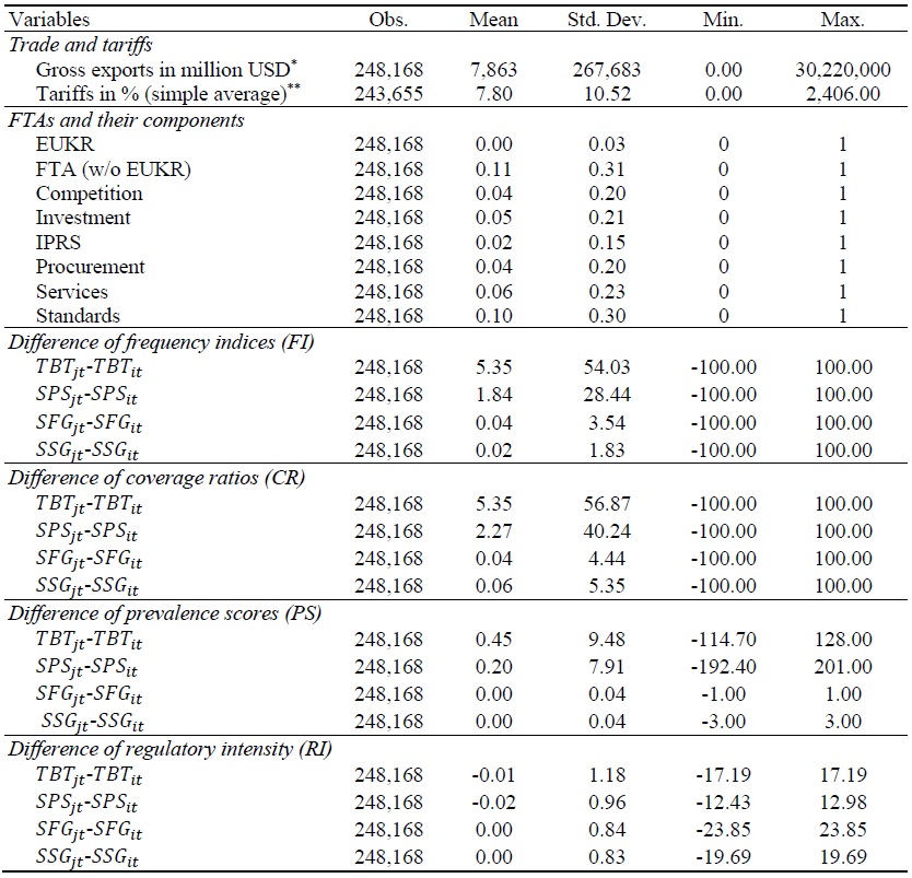
For each of the five types of NTMs, we calculated bilateral annual frequency indices (FI), coverage ratios (CR), prevalence scores (PS) and regulatory intensity (RI) indicators, which enter our subsequent structural gravity model estimation (Table 3). The FI and CR range between 0 and 100. For contingent protection measures and SSG, mean values are well below 1. For TBTs and SPS measures, they range between 11 and 35, i.e., across all country pairs and years (1995-2017) roughly 34% of products and 35% of import volumes were affected by TBT, while 11% of product lines and 15% of import flows were subject to SPS.
The minimum of the PS is also zero, however its maximum is not pre-defined. It can be interpreted as an FI scaled by the number of NTM regulations applicable. For contingent protection measures, values are almost identical to the FI, as multiple ADP/CVD/SSG per 6-digit product would be applicable only if several products at a more detailed product level (e.g. 12-digit) were subject to measures. The situation is very different for SPS measures and TBTs. The same product may be subject to labelling requirements, authorisation requirements, tolerance limits for residues of substances (e.g. pesticides), mandatory tests, certificates etc. This boosts the mean PS for TBTs to 291 and the mean PS for SPS measures to 153, with maximum values exceeding 10,000 for both NTM types.
The RI can be positive if the number of NTMs a product
The CR provides interesting and easily understandable descriptive insights. However, it suffers from an endogeneity bias when used for econometric analysis, as quasi-prohibitive NTMs reduce the volume of imports of the affected product. The RI aims to correct this shortcoming by weighting the NTM counts by the share of imports of product
The following figures represent simple averages across countries and show that the interpretation of the evolution of NTMs may differ significantly by indicator. Throughout, we show SPS and TBTs in one graph and group the remaining trade defence and agricultural measures together.
Frequency indices grew strongly for TBTs and SFG. SPS measures grew steadily as well, but not as fast as TBTs. No clear trend is visible for ADP, CVD and SSG.
Coverage ratios, which take affected trade volumes into account, reduce the gap between TBTs and SPS measures through a stronger uptick of the latter. They dissolve the upward trend of SFG, which display a higher volatility. Although frequency indices give the impression that SFG are by far the most important contingent NTMs, coverage ratios indicate that ADP and SSG are equally important.
Prevalence scores, which weigh frequency indices not by trade volumes but by the number of notifications applicable to the same product, suggest that the wedge between TBTs and SPS measures has strongly increased since about the year 2010. The rescaling of the PS also makes SFG and SSG look much more alike.
Finally, regulatory intensities show mainly positive values for TBTs, SFG and SSG, but negative scores for SPS measures, ADP and CVD. The average across imposing economies can be negative, especially when the measure is used only by a few economies or if some countries use the instrument very intensely, which pushes up the mean.
1)See e.g.,
2)See
3)A detailed classification of types of NTMs, including examples, is provided by
4)The first version of this data was produced as part of the project PRONTO (Productivity, Non-Tariff Measures and Openness) under the European Union’s Seventh Framework Programme under grant agreement no. 13504 and has been documented in
5)Exceptions include work by
6)Further measures that aim to capture the intensity of NTMs’ use and their price and quantity impacts are currently evolving in the international trade literature. Different econometric methods are used to translate NTMs into ad valorem equivalents that can be understood as the impact of NTMs on import prices, which are in turn more comparable to tariffs. These are derived either through direct observations of price changes (e.g.
7)There are some limitations to the stock variable, as the date of withdrawal of NTMs is often not available, resulting in stock figures that are too high.
8)We would like to stress for readers who are familiar with the indicators presented by
9)WTO document G/TBT/M/79 referring to G/TBT/N/KOR/817.
10)WTO document G/ADP/N/335/KOR: Finland: coated printing paper; France: butyl glycol ether; Italy and Spain: stainless steel bars.
11)WTO document G/ADP/N/335/EU.
12)See
II. Evaluating the Value added of NTMs in Trade Policy Analysis
The European Commission distinguishes four different types of FTAs. Most EU-FTAs in force are so-called first-generation FTAs, which were concluded prior to the announcement of the EU’s Global Europe strategy (EC, 2006). Economic Partnership Agreements (EPAs) were established with African, Caribbean and Pacific (ACP) economies to address special development needs. Deep and Comprehensive Free Trade Areas (DCFTAs), in contrast, focus on Europe’s neighbourhood. Finally, second-generation – or new-generation – agreements are deep reciprocal FTAs that extend much further than tariff concessions, touching upon topics such as competition, intellectual property rights, sustainable development and standards.
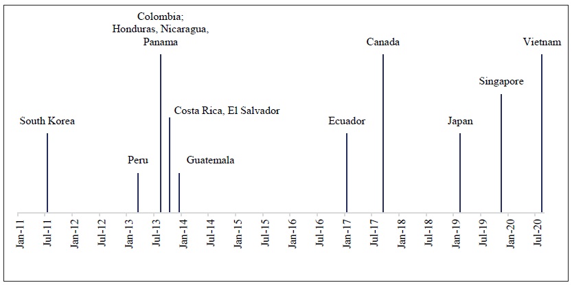
The EU-KR agreement was the very first of the EU’s second-generation agreements and hence served as a benchmark for future agreements (Figure 4). Between 2013 and 2017, agreements with nine economies in Central America or in the Andean Community started to apply. The trade part of the Comprehensive Economic and Trade Agreement (CETA) with Canada has provisionally been applied since 21 September 2017. Japan and Singapore followed suit in 2019 and Vietnam in 2020.
NTMs feature prominently in these agreements. Separate chapters are devoted to SPS measures and TBTs. In this context, the text analysis performed by Allee et al. (2017) for EU agreements with Canada, Central America, Singapore and South Korea suggests that new-generation trade agreements do not push for harmonisation towards European standards but rather for establishing an equivalence of differing rules or agreement on international standards.
Depending on the bargaining power of trading partners, agreement on common standards may result in upgrading or downgrading of standards. Aisbett and Silberberger (2020) suggest that trade liberalisation – e.g., through the establishment of FTAs – fuels divergence between countries: Economies with many SPS measures in place follow a race to the top after further trade liberalisation, while economies with fewer SPS regulations tend to lower their notification rates. The former fits the picture drawn for SPS measures and TBTs notified to the WTO: The EU is among the heaviest users of these standard-like NTMs, and so are many trading partners with which the EU has established second-generation FTAs (Figure 5).
1. EU-South Korea FTA: Ex-ante Analyses
Given the novelty of the EU second-generation agreement type, there was great interest in estimating ex-ante the potential impact of the EU-KR agreement. Negotiations for the agreement were launched in May 2007. It was signed in October 2010, the European Parliament gave its consent in February 2011, paving the way for the provisional application of the agreement as of July 2011, including all trade-related provisions. It fully entered into force in December 2015.
Francois et al. (2007) applied a computable general equilibrium (CGE) model to test two scenarios of the EU-Korea agreement, which they compared to a ‘full FTA’, where all bilateral tariffs (including those on food products) were abolished and trade in services was also fully liberalised. The first scenario assumed tariff reductions of 40% in the food sector, full bilateral reductions in the non-food sectors and a 25% reduction in trade barriers applying to the services sectors. In the second scenario, a reduction of barriers hampering international trade in services by 50% was assumed. Francois et al. (2007) did not model reductions in NTMs, but mentioned that in some sectors, such as the automotive sector, these were more important than tariffs. Their results suggested that South Korea was set to gain more from the trade agreement than the EU, because it was less integrated into international trade before the agreement. In relative terms, South Korea’s real income was estimated to increase by 0.58% in the first scenario and by 1% in the second scenario. Expected real income growth for the EU was calculated to be significantly lower, at 0.01% in the first scenario and 0.03% in the second scenario. For the hypothetical case of full trade liberalisation, their model suggested gains at 0.05% of GDP for the EU and 2.3% for South Korea.
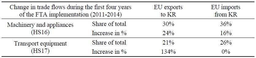
Another quantitative assessment was provided by Decreux et al. (2010), who included reductions of NTMs in their calculations. They found that trade protection via NTMs exceeded tariff protection and that NTM protection by South Korea was higher than in the EU, notably for textiles, machinery and (especially) cars. Decreux et al. estimated GDP effects for the EU and South Korea in the order of 0.08% and 0.84%, respectively. Relative gains from free trade were thus expected to be about ten times higher for South Korea than for the EU, almost proportionate to the respective sizes of their economies.13 However, bilateral exports of the EU were expected to rise by 82.6%, compared with an estimated increase of 38.4% in South Korean exports. Exceptionally high gains for the EU of about 400% were predicted for exports of cars and trucks to South Korea. In fact, exports of motor vehicles to South Korea increased by more than 200% and imports by about 50% in the first four years of the FTA’s implementation (EC, 2016).
2. EU-South Korea FTA: Ex-post Evidence
Since then, some ex-post evaluations have been conducted, all of which showed that EU exporters gained more than South Korean ones.
Civic Consulting and the Ifo Institute prepared a report for the European Commission (EC, 2018). It showed that trade between the two partners increased, although very unequally: EU exports to South Korea rose by 54% as a result of the agreement, while South Korean exports to the EU grew only by 15%. This result is based on trade data from the World Input-Output Database (WIOD),14 covering the years up until 2014. The results derived from a CGE model suggested that the GDP of the EU increased by 0.03% because of the FTA. The GDP gain for South Korea was evaluated to be significantly higher, at 0.3%. The authors, however, stressed that these estimates constituted the lower bounds of the true economic effect. Altenberg et al. (2019) confirm this finding. Their gravity model estimation indicates that the FTA increased trade flows between the EU and South Korea by 36%.
Evaluating the extensive and intensive margin of trade along different stages of the agreement – from the start of negotiations to its implementation – Lakatos and Nilsson (2017) found for the EU that the probability of exporting, as well as the value of exports, increased by about 10% as a consequence of the agreement. For South Korea, they reported lower magnitudes. Their analysis for South Korea suggested a 4.9% increase in the probability of exporting and a 2.2% increase of export volumes to the EU. They explained the asymmetry of effects by the differences in the initial policy environment of the two trading partners, arguing that EU exporters had more to gain in terms of decreasing tariffs and increasing the predictability of South Korean trade policy. Notably, before the FTA was applied, 68% of the value of South Korean exports entered the EU duty free, while only 15% of EU exports to South Korea faced zero tariffs.
Focusing on the automotive industry, Juust et al. (2020) found that the EU-KR agreement had a significant positive effect on bilateral trade (+93%). They attribute this finding to the initially high level of NTMs that existed in the automotive sector, which the FTA significantly reduced. However, when considering total trade, the results from the gravity regression show only a small positive and not statistically significant effect. Allowing the EU-KR dummy variable to differ by the direction of the trade flow, they confirmed that total exports from the EU to South Korea significantly increased, but exports from South Korea declined.
Both EU exports to as well as imports from South Korea are dominated by two product groups: machinery and appliances, and transport equipment (Table 4). During the first four years of the application of the agreement, EU exports in the transport sector grew by more than 130%, driven by motor vehicle exports (HS 8703), which increased by 206% in volume. Even when overall exports stagnated in 2018 (Figure 6), EU exports of passenger cars continued to grow by 9%, and hence transport sector exports from the EU to South Korea overall increased by 187% since the agreement began to apply (EC, 2019). A survey conducted in 2015 suggests that the extraordinary performance of EU exports was largely driven by broad economic and social trends, including the fast maturing of the South Korean economy, resulting in a quickly growing need for high-end industrial goods and also increased purchasing power for South Korean consumers (Cherry, 2018).
However, not every EU member took advantage of FTA preferences. The preference utilisation rate within the EU ranged between 6% and 91%, with the highest rates (above 80%) found for Latvia, Austria and Slovakia, and the lowest rates (below 16%) observed for Malta and Luxembourg (EC, 2016). The preference utilisation rate of South Korean exports to the EU increased from 85% in 2015 to 88% in 2018. During this period, the preference utilisation rate of EU exports to South Korea increased from 68% to 81% (EC, 2019).
The development of trade flows and preference utilisation rates, as well as activities of specialised committees set up to implement the FTA is presented by the European Commission on an annual basis (EC, 2016, 2017). With regard to NTMs, the report of 2016 highlighted consultations in the Committee on Sanitary and Phytosanitary Measures regarding a Korean import ban on pork from Poland and poultry from multiple EU Member States. The approval of beef imports from some EU Member States is still pending (EC, 2019). Separate working groups were established for motor vehicles, as well as pharmaceuticals and medical devices.
Prior to the establishment of the EU-KR FTA, foreign executives and officials raised concerns that as one non-tariff barrier imposed by South Korea was eliminated, one or more might appear in its place. Interview results suggest that these negative expectations were partly fulfilled; in addition, the willingness to dismantle non-tariff trade barriers has decreased in line with the growing trade deficit South Korea experienced with the EU (Cherry, 2018).
3. Data: The Trade Policy Toolkit
Information on regional trade agreements (RTAs) is available via the WTO RTA database. All notified RTAs, distinguished by type (e.g. free trade agreement, customs union, economic integration agreement or partial scope agreement), were provided by Egger and Larch (2008) and updated in 2018.
As indirect measures of NTMs, we make use of a dataset using indices for the depth of FTAs.15 The Design of Trade Agreements (DESTA) dataset coded around 100 items in more than 1,000 trade agreements for the period 1948-2018 (Dür et al., 2014; data updated in 2019). We use coded information on seven components of FTAs: tariff reductions, regulations on competition, agreements on intellectual property rights (IPRS), aspects of investments, public procurement, services and standards. We are particularly interested in the standards component as it focuses on SPS measures and TBTs and might therefore serve as the closest proxy for observed NTMs.
For direct information on NTMs, we will focus on the wiiw NTM data based on WTO I-TIP and TTBD, enhanced by product code matching (Ghodsi et al., 2017 and Grübler and Reiter, 2020). These data are further transformed to indices (FI, CR, PS and RI), as described in previous sections. Respective summary statistics were presented in Table 3 in Section I. Summary statistics on other variables used for the econometric analysis can be found in the appendix.
Despite their declining role, particularly among industrialised countries and nonagricultural goods, tariffs remain an important part of trade policy. Our main sources for tariffs data are the Trade Analysis Information System (TRAINS) database and the WTO Integrated Data Base (IDB), provided via the World Integrated Trade Solution (WITS) platform of the World Bank. If applicable and available, effectively applied tariff rates entered our dataset. Otherwise, we referred to preferential tariff rates or most-favoured-nation tariff rates. We consider simple averages over tariffs reported at the HS 6-digit level, as trade-weighted tariffs would suffer from an endogeneity bias.
For trade data, we consult two different data sources: Our main specification relies on trade data provided via the UN Commodity Trade Statistics Database (UN Comtrade). It covers a long time span (1996-2019) and a large set of countries16 but is unbalanced and approximations of intra-national trade flows are necessary. These intra-national flows are goods produced and consumed in the same country, which are important for arriving at unbiased gravity estimates (Yotov et al., 2016). These are computed by subtracting the sum of exports from countries’ gross output taken from national accounts provided by the UN.17 The availability of this data restricts our sample to the period 1996-2017.
For robustness checks, we refer to the World Input-Output Database (WIOD),18 published by Timmer et al. (2015, 2016). Based on their methodology, the dataset was complemented by Reiter and Stehrer (2018) to cover more countries, particularly in the Western Balkans region. The wiiw Europe Integrated Input-Output Database covers 50 countries and 32 industries for the period 2005-2014 and has the advantage of providing information on intra-national trade at the sectoral level. The inherent disadvantage of this data source is that it covers only four years since the application of the EU-KR agreement.
4. Gravity Model Estimation
Starting with Jan Tinbergen in 1962, the gravity model of international trade shows in its simplest form that trade flows
Since the seminal work by Anderson and van Wincoop (2003), which laid the theoretical foundations for the gravity model, it has developed to be the workhorse for the analysis of international trade flows and trade policies and has seen several econometric improvements. There is a vast literature on the evolution of the model to a structural gravity model, with best practices on employing the theoretically founded gravity equation summarised by Bacchetta et al. (2012) and Yotov et al. (2016). We use the Poisson Pseudo Maximum Likelihood (PPML) estimator to derive our results. The first specification of the structural gravity equation we employ takes the following form:

Our dependent variable  refers to simple averages of bilateral tariffs between countries
Multilateral resistance terms (MRTs) account for the fact that the impact of bilateral policies between two countries depends on which policies the trading partners have in place with the rest of the world. For example, if we want to evaluate the effect of an FTA between the EU and South Korea, it is crucial to account for their trade ties with other economies. These MRTs are proxied by time-varying exporter fixed effects
Country-time fixed effects account for country specifics, which can change over time, for example, GDP, population size, level of development (Olivero and Yotov, 2012). Country-pair fixed effects absorb time-invariant information such as distance between trading partners, past colonial ties, common borders or common language, and help to reduce the linkages between endogenous trade policy instruments and the error term, as stressed by Baier and Bergstrand (2007). With this array of fixed effects in place, the coefficients of FTAs only capture the effect of trade agreements that have been put in place between 1996 and 2017.
In a second specification, we include NTM

NTM
This approximation of the regulatory gap has the disadvantage of not capturing levels. As such, the difference between two countries with low NTM indices may face a similar gap as a country pair where both countries exhibit high values for respective NTM indices. For this reason, we employ an alternative multiplicative specification in the robustness section. It has the merit of clearly distinguishing country pairs with high NTM indices from those with low NTM indices but lacks the feature of a regulatory gap that proxies for similarities of trading partners with respect to the application of non-tariff policy.
13)According to the World Development Indicators, in 2011 the EU’s GDP amounted to USD 15.7 trillion, compared with USD 1.3 trillion for South Korea (i.e. approximately 8% of that of the EU). Similarly, the EU had 440.7 million inhabitants, compared with 49.9 million in South Korea (i.e. 11% of the population size of the EU).
14)See
15)Another interesting data source is the Trade Agreement Heterogeneity Database (TAHD) by
16)We use trade data from a large set of countries, which allows us to estimate the fixed effects (exporter-year, importer-year, country-pair) as accurately as possible rather than restricting our data sample to trade data between South Korea and the EU. Consequently, the NTM data also has to cover as many countries as possible to not run into problems related to omitted variables.
17)The UN collects these data:
18)See
19)Croatia joined the EU in 2013. Hence, the EUKR dummy variable for Croatia-South Korea observations switches to 1 in 2014.
20)This approach was also employed for the evaluation of the implementation of the EU-South Korea agreement prepared by Civic Consulting and the Ifo Institute for the European Commission
21)When effectively applied tariffs were not available, we referred to preferential tariff rates and subsequently to most-favoured-nation tariff rates.
22)
23)A related bilateral measure is the distance in regulatory structure introduced by
III. Empirical Results
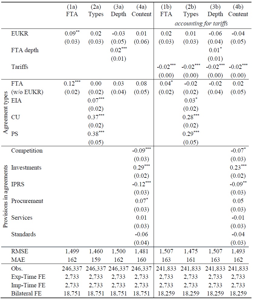
Results of our first specification are presented in Table 5. The simplest form is given in column 1a with a dummy variable for the EU-KR FTA and an additional indicator variable for all other worldwide trade agreements based on Mario Larch’s Regional Trade Agreements Database (Egger and Larch, 2008). As this database distinguishes multiple types of agreements with differing degrees of trade and political integration, column 2a shows the results when we account for the difference between free trade agreements (FTAs), economic integration agreements (EIAs), customs unions (CUs) and partial scope agreements (PSs), which cover only certain products. Similar specifications were presented in the evaluation report of the EC (2018), prepared by Civic Consulting and the Ifo Institute, on the implementation of the EU-KR FTA. Column 1 indicates that the EU-KR FTA increased trade by [exp(0.09)-1]x100 = 9.42%. When controlling for different trade agreement types in column 2a, the most effective trade agreement types were customs unions and partial scope agreements, while the coefficient on the EU-KR FTA becomes insignificant. Such a change was not reported in the evaluation of the European Commission, which was restricted to the years 2000-2014 and based on WIOD data.
Although column 1a provides us with information on trade increases after the establishment of the EU-KR FTA, we cannot learn which trade policy areas were driving the result. Therefore, we make use of a different dataset for columns 3a and 4a, namely the Design of Trade Agreements (DESTA) database compiled by Dür et al. (2014), updated in 2019. It allows for the differentiation of trade agreements by their depth (column 3a), or by the trade liberalising provisions incorporated in FTAs (column 4a). As outlined in the descriptive section, the agreement with South Korea is truly comprehensive, includes sensitive economic areas and remains among the deepest agreements that the EU has in place. Results based on the depth indicator suggest that deeper FTAs tend to increase trade significantly. If the depth of an agreement increases by one, trade is expected to increase by [exp(0.02)-1]x100 = 2%. The EU-KR FTAs is coded with a depth of 7, meaning that a switching from 0 to a depth of 7 increased trade by 14%. When considering the content of these agreements (summarised in the depth indicator), it seems that public procurement rules and provisions on investments have a significant positive impact on bilateral trade, while FTA components addressing competition and intellectual property rights (IPRS) on average reduce trade. Although goods and services trade are partly complementary, FTA regulations on services on average do not appear to have a significant impact on goods trade. Finally, the coefficient on standards – relating primarily to SPS measures and TBTs – is negative and not significantly different from zero.
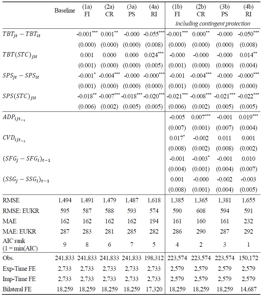
Columns 1b to 4b replicate the first four estimations, but additionally include tariffs, such that all other control variables showing a positive trade effect are attributable to non-tariff policies. As expected, higher tariffs are associated with lower trade flows. Results on trade agreement types, their depth and provisions remain almost unchanged. In addition, for all specifications explicitly accounting for tariffs, the variable capturing the EU-KR agreement is insignificant, adding no extra information. This suggests that the effects of the EU-KR agreement can be sufficiently described by the increases in depth, reductions in tariffs and the provisions common in deep FTAs.
Henceforth, the specification presented in column 4b, which covers the specificities of trade agreements in greatest detail, features as our baseline for further analysis on NTMs.
In Table 6 we first incorporate standard-like NTMs, i.e., SPS measures and TBTs as well as associated specific trade concerns (STCs), measured by frequency indices, coverage ratios, prevalence scores and regulatory intensity indicators.24 Except for prevalence scores, indicators for NTMs show significant negative impacts of bilateral differences in TBTs and SPS measures. This finding is in line with our hypothesis that a higher level of regulation by the importing economy relative to the exporting economy reduces bilateral trade flows. Furthermore, regulations related to human and plant health, against which trading partners have raised concerns (SPS(STC)), exhibit a particularly negative effect.
These four specifications were re-estimated by additionally considering bilateral antidumping and countervailing measures as well as unilateral safeguards and special agricultural safeguard measures. Counteractive measures constitute a reaction to import surges,25 thus we include them with a lag of one year to reduce the inherent endogeneity bias. In the sensitivity analysis (presented in Table 7) we also consider results without lags. The inclusion of these variables changes the component of trade agreements designated for competition issues to become insignificant. Coefficients on standard-like NTMs remain essentially unchanged. However, the coefficients on the counteracting measures themselves are not conclusive, showing changing signs and significance levels across indicators.
For the comparison across NTM indices, we need to bear in mind the caveat of the coverage ratio suffering from endogeneity bias, as it is a trade-weighted measure. Trade weights used for the regulatory intensity measures are product and not country-pair specific. Endogeneity at the bilateral level should thus be less of concern. Nonetheless, we refer to the prevalence score and the frequency index, which do not incorporate any trade weights, for the sensitivity analysis. We present two tables to assess the robustness of our findings. First, we alternate our variable specifications (Table 7). Second, we use trade data from the wiiw Europe Integrated Input-Output Database instead of UN Comtrade (Table 8).
The first column of Table 7 replicates our findings using prevalence scores from Table 6. In the second column, we dropped the lag from counteractive measures, restoring the significance of the negative coefficient on competition while leaving all coefficients on contingent protection measures insignificant. Column 3 varies from our baseline as unilateral NTMs do not enter the regression as differences between the exporter and the importer level of the NTM indicator, but as a product. This specification changes the negative coefficient on SPS measures to become significant and special safeguards to become strongly negative and highly significant. This result suggests that the level of unilateral NTMs, which are designed to protect the domestic markets from a drop in prices or a strong import influx in the agricultural sector, should not be neglected. In column 4 we create two-year periods and use the average trade flows as dependent variable.26 Real-valued independent variables are also averaged; for dummy or integer variables we use the minimum of the two-year period. This modification boosts the positive effect of the investment variable and tariff liberalisation but results in a strong negative trade effect associated with the EU-KR FTA. This may be due to the stagnant goods exports of South Korea to the EU, which are attributed a bigger weight when two-year averages are considered. Finally, restricting the analysis to trade flows exceeding one million USD to reduce the volatility of trade flows does not change our baseline results. SPS (STC) is the only NTM to show consistent results across all five specifications: its coefficient is negative and statistically significant. This finding underlines the difficulties for exporters to meet health related standards of importers.
As an alternative to UN Comtrade data, analyses can be performed on datasets based on input-output tables, such as WIOD (Timmer et al., 2016). The latter has been used, for example, in the most recent assessment of the EU-KR agreement by the EC (2018). The fact that trade flows are balanced,27 the possibility of including services trade and the availability of intra-national flows are the main advantages of this dataset. On the other hand, its two major drawbacks are that it stops in 2014 (one year before the EUKR FTA entered fully into force) and that its country coverage is smaller. The wiiw Europe Integrated Input-Output Database includes additional countries in the Western Balkans (Reiter and Stehrer, 2018). Moving from UN Comtrade to the wiiw Europe Integrated Input-Output Database reduces the number of country-pairs from more than 18,000 to about 2,500 (Table 8). As many countries are aggregated in the ‘rest of the world’, many trade policy variables cannot be appropriately applied.
Looking at total bilateral trade, the use of the input-output database reduces the significance levels of provisions covered in trade agreements as the country coverage and the shorter time span significantly reduce the number of deeper FTAs for which provisions beyond tariff cuts could be assessed. However, it retains the significantly negative effect associated with SPS measures that triggered complaints, SPS (STC).
Splitting trade flows further into agriculture and mining on the one hand, and manufacturing on the other, reveals that the biggest positive effects of the EU-KR FTA concern the former. This is in line with our earlier descriptive analysis showing that the EU-KR trade links in the agricultural and food sector were characterised by particularly high levels of protection prior to the establishment of the FTA.
Competition rules have on average a negative impact on trade in agriculture and mining, but a positive effect for the manufacturing sector. Negative effects for both product groups are found for IPRS. For the agriculture and mining group, positive effects are suggested for investment regulations, public procurement rules and agreement on standards, while differences in SPS indicators exhibit a negative coefficient. Effects of contingent protection measures are relatively bland except for countervailing duties, the trade effects of which appear negative and highly significant for the manufacturing sector.
Results using the traditional frequency indices or prevalence scores show the same overall findings, with one notable exception: frequency indices suggest a negative trade effect arising from differences in trading partners’ TBT levels in the manufacturing sector, while a positive significant effect is implied by regression analysis using prevalence scores.
To sum up, the EU-KR FTA dummy variable is positive when no other components of deep FTAs are accounted for. The included FTA provisions, together with the tariff variable, seem to explain the positive effects of signing an FTA for the most part. The statistically insignificant coefficient for the EU-KR FTA means that there is no
Investment provisions in FTA treaties tend to significantly increase trade flows, while countries that have included IPRS provisions in their FTA treaties seem to experience lower trade flows. TBTs and SPS measures show mostly negative coefficients, which are, however, not always significantly different from zero. Particularly eye-catching are the negative trade effects of SPS measures that have been the subject to complaints to the WTO. The way in which product level information on NTMs is aggregated to bilateral trade flows (through frequency indices, coverage ratios, prevalence scores or regulatory intensities) does not have a strong influence on the results, despite the fact that their evolution over time varies considerably.
24)The number of observations for the regulatory intensity is lower than for the other indicators because there are products for which not a single NTM applied. Thus, we cannot compute the regulatory intensity for those product-NTM combinations as this would lead to a division by a standard deviation of 0. Observations with undefined regulatory intensities drop out.
25)See, for example,
26)
27)Balanced trade flows mean that reported exports of country
IV. Conclusion
The number of free trade agreements (FTA) and the topics covered therein are rising. New-generation agreements of the EU following its Global Europe strategy in 2006 are more ambitious in the areas of non-tariff measures (NTMs). These are becoming increasingly important and are replacing tariffs at the core of trade agreements among industrialised economies. Correspondingly, there is a growing interest in related research, and various methods for measuring NTMs and their effects are developing.
This paper aims to contribute to this growing literature by applying several frequently used indices for NTMs found in the literature to the same country sample and trade policy datasets, thereby assessing their ability to improve predictions of trade flows. It describes NTMs applied between the EU and South Korea, for which the first new-generation FTA has been provisionally applied since 2011 and entered into force in 2015.
The descriptive analysis of notification data for the EU and South Korea reveals that the policy mix applied to bilateral trade relations differs widely. While the EU resorts to antidumping and countervailing duties, primarily targeting the manufacturing sector, South Korea makes more frequent use of bilateral sanitary and phytosanitary measures for animal and vegetable products. Both trading partners have reduced their use of agricultural safeguards – mainly addressing sugar and meat products in the case of the EU, but vegetable and plant products in the case of South Korea.
The information on components of FTAs as provided by the Design of Trade Agreements (DESTA) database proved particularly useful in the econometric analysis. Results suggest that investment provisions significantly influence trade flows positively, while IPRS seem to hamper trade. The robust negative effect of tariffs points to the fact that tariffs continue to be an important trade policy tool.
The evolution of bilateral frequency indices, coverage ratios, prevalence scores and regulatory intensity measures of NTMs convey distinct messages. Indicators are strongly increasing over time for TBTs, and faster than SPS measures. The latter seem to be driven by a number of heavy users, resulting in on average negative regulatory intensity scores. Upward trends are also observable for (agricultural) safeguard measures.
In the regression analysis, the four indices show similar coefficients and behaviour across all tested specifications for standard-like NTMs but are inconclusive on the aggregate level for counteracting measures. SPS measures against which trading partners have filed a specific trade concern at the WTO seem to exert the biggest negative impact on trade flows.
To conclude, the EU’s first deep and comprehensive second-generation trade agreement with South Korea constitutes a milestone in EU trade policy. Tariffs on the majority of traded goods were eliminated after the agreement started to provisionally apply in 2011. The agreement covers sensitive policy areas reaching far beyond tariff liberalisation, such as services trade, investment, TBTs and SPS measures. Tariff cuts and information on FTA provisions provided by DESTA explain the positive trade effect associated with the EU-KR FTA. However, the descriptive and econometric analyses suggest that some high trade costs associated with NTMs prevail. Future cooperation could be particularly promising in the area of sanitary and phytosanitary measures.
Tables & Figures
Table 1.
NTM Indicators under Review
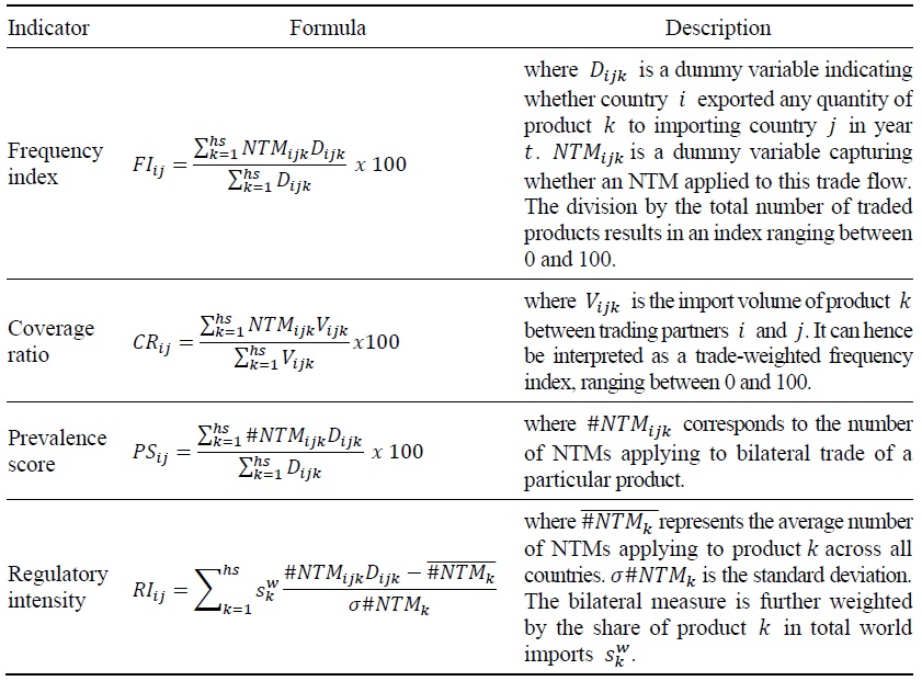
Figure 1.
Types of Bilateral NTMs Applying between the EU and KR
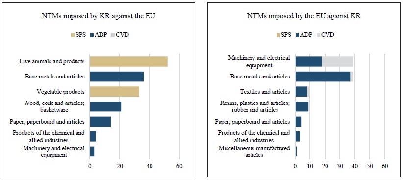
Note: Product descriptions refer to sections of the Harmonised System (HS).
Sources: wiiw NTM Data based on WTO I-TIP and TTBD (1995-2019); authors’ calculations.
Table 2.
Potential and Actual Application of SSG by South Korea and the EU
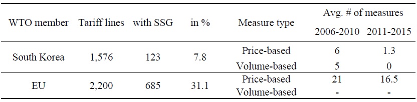
Source:
Table 3.
Summary Statistics for Indicators across NTM Types
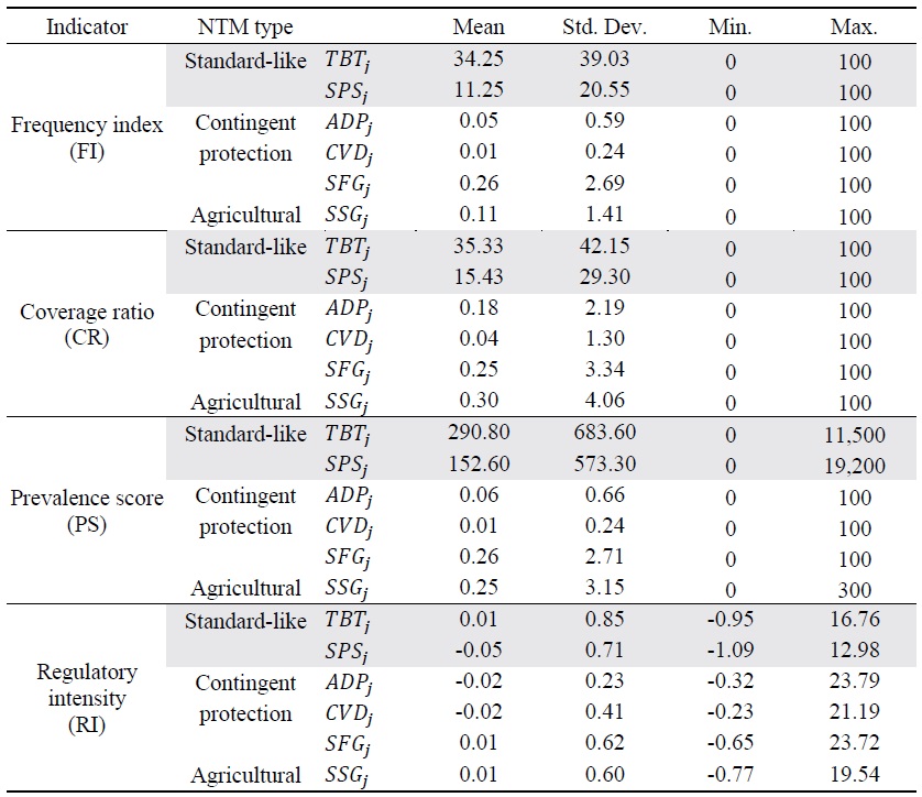
Sources: wiiw NTM Data based on WTO I-TIP and TTBD (1995-2019); authors’ calculations.
Figure 2.
FI and CR across NTM Types over Time, Average across Imposing Economies
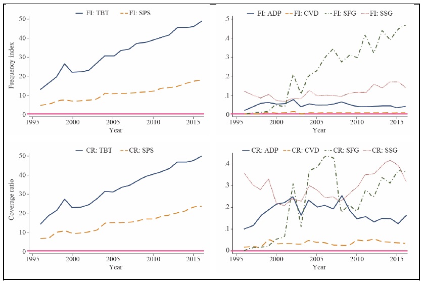
Notes: Simple average across all importer-exporter country pairs. EU measures are assigned to every EU Member State.
Sources: wiiw NTM Data based on WTO I-TIP, TTBD; authors’ calculations.
Figure 3.
PS and RI across NTM Types over Time, Average across Imposing Economies
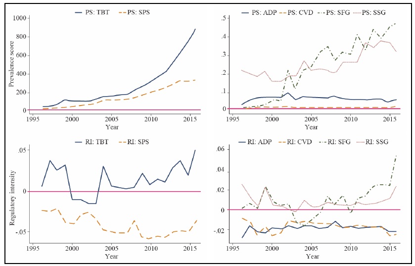
Notes: Simple average across all importer-exporter country pairs. EU measures are assigned to every EU Member State.
Sources: wiiw NTM Data based on WTO I-TIP, TTBD; authors’ calculations.
Figure 4.
Second-generation EU Trade Agreements
Sources:
Figure 5.
Top 20 SPS- and TBT-Imposing Economies Sum of Notifications for the Period 1995-2019
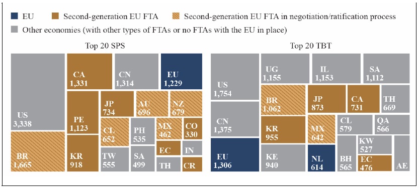
Note: EU Member States and the EU as a whole are members of the WTO and are considered separately in the chart.
Sources: wiiw NTM Data based on notifications to the WTO; authors’ illustration.
Table 4.
Machinery and Transport Equipment Account for more than Half of EU-KR Trade
Source:
Figure 6.
Evolution of EU-28 Trade in Goods with South Korea (in billion USD)
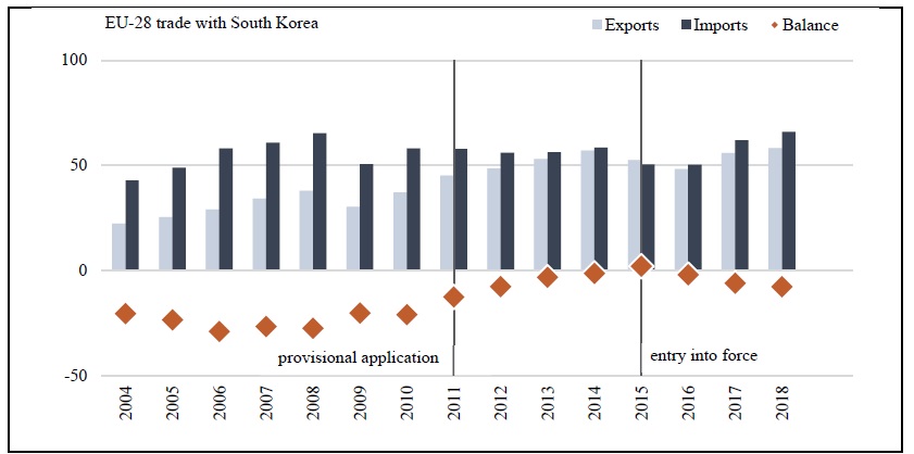
Sources: UN Comtrade; authors’ illustration.
Table 5.
Estimates of Trade Effects of the EU-KR FTA: 1996-2017
***p < 0.001; **p < 0.01; *p < 0.05
Table 6.
Trade Effects of FTAs Accounting for NTMs: 1996-2017
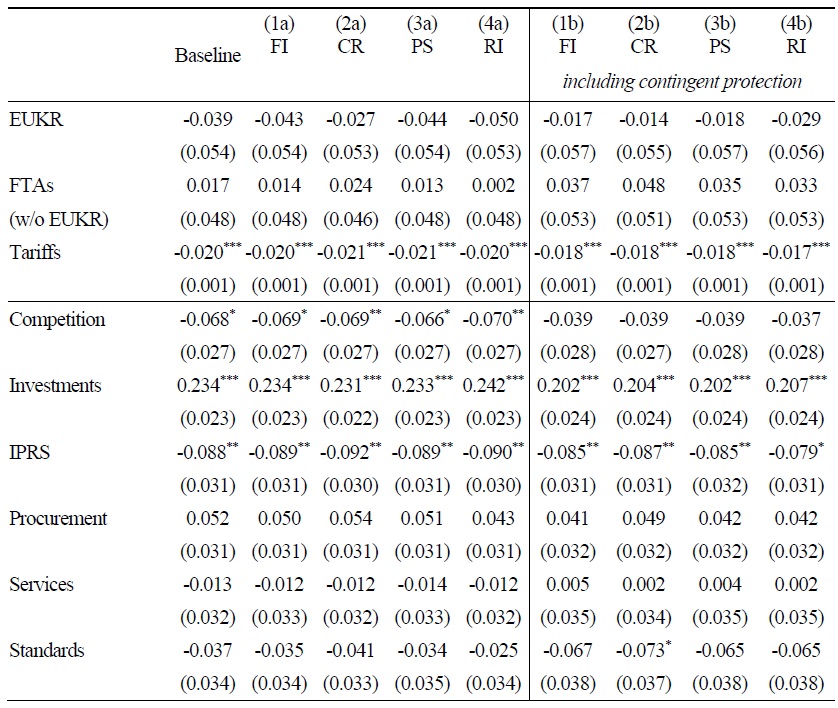
Table 6.
Continued
***p < 0.001; **p < 0.01; *p < 0.05
Table 7.
Robustness Table Using Prevalence Scores (PS): 1996-2017
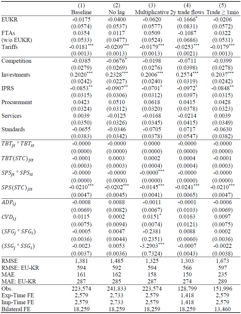
***p < 0.001; **p < 0.01; *p < 0.05.
Note: Baseline refers to column 3b in
Table 8.
Robustness Table Using WIOD
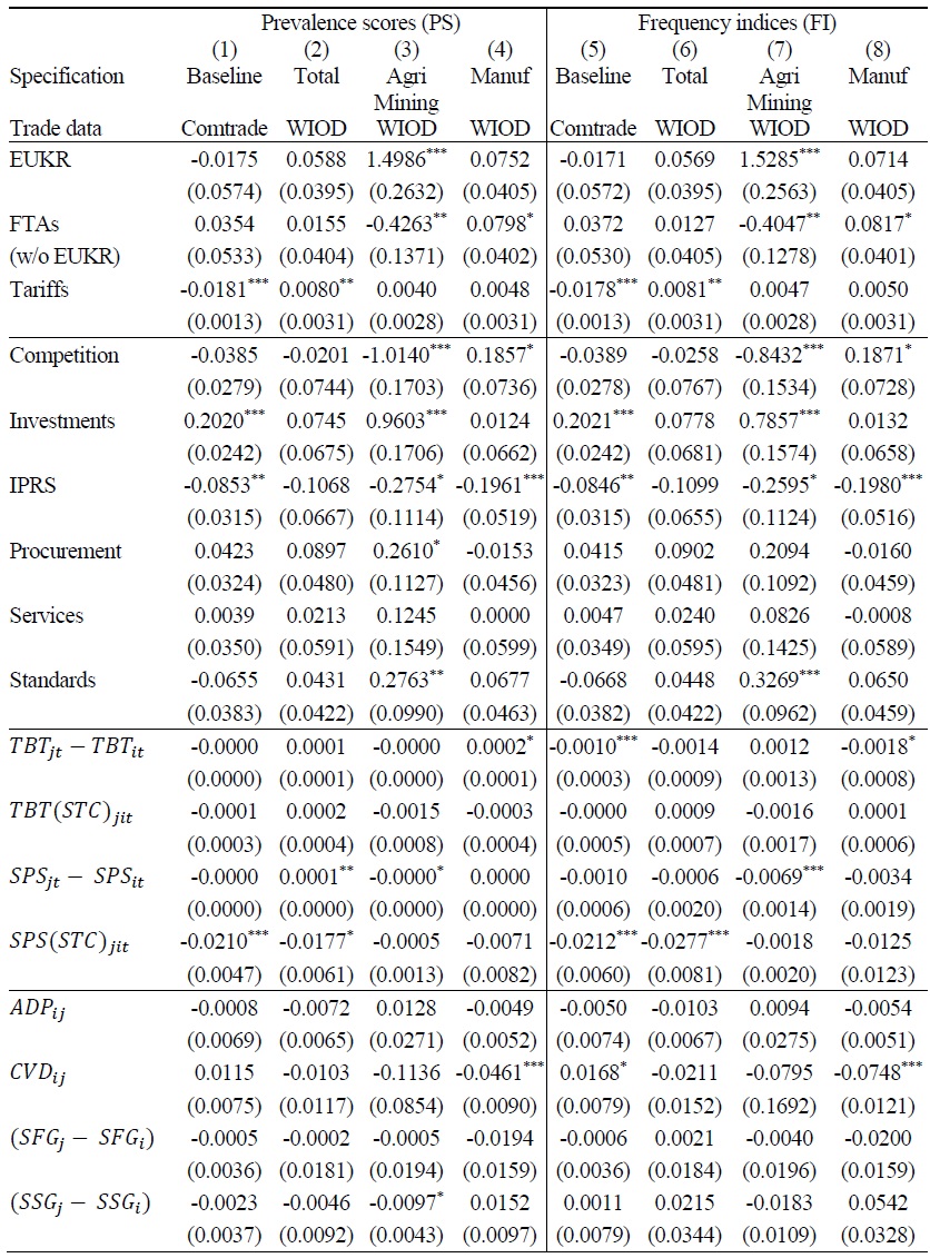
Table 8.
Continued
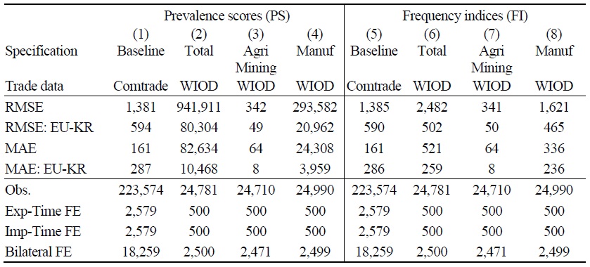
***p < 0.001; **p < 0.01; *p < 0.05.
Notes: Baseline refers to columns 1b and 2b in
APPENDIX: SUMMARY STATISTICS
Table 3 in Section I provides summary statistics for various NTM types and indicators: frequency index (FI), coverage ratio (CR), prevalence score (PS) and regulatory intensity (RI). The following tables provide summary statistics on the remaining variables used in the main specification of the econometric analysis as well as the proxy for regulatory gap measures for unilateral NTM types.
Appendix Tables & Figures
* As outlined in the data section, bilateral trade flows provided by UN Comtrade are complemented by intra-country trade flows computed by subtracting the sum of exports from countries’ gross output, taken from national accounts provided by the UN.
** There are three observations of average tariffs exceeding 300%. According to UN TRAINS, simple averages of applied tariffs and most-favoured nation tariffs employed by Egypt against Armenia amounted to 1,203% in 2013, against the Bahamas to 1,203% in 2012 and against Bermuda to 2,406% in 2012.
References
-
Aisbett, E. and M. Silberberger. 2020. “Tariff Liberalization and Product Standards: Regulatory Chill and Race to the Bottom?”
Regulation & Governance . forthcoming. <https://doi.org/10.1111/rego.12306 > (accessed October 21, 2020) -
Allee, T., Elsig, M. and A. Lugg. 2017. “Is the European Union Trade Deal with Canada New or Recycled? A Text-as-Data Approach,”
Global Policy , vol. 8, no. 2, pp. 246-252.
-
Altenberg, P., Berglund, I., Jägerstedt, H., Prawitz, C., Stålenheim, P. and P. Tingvall. 2019.
The Trade Effects of EU Regional Trade Agreements – Evidence and Strategic Choices . Kommerskollegium (National Board of Trade Sweden) eBook. <https://www.kommerskollegium.se/en/publications/reports/2019/the-trade-effects-of-eu-regional-tradeagreements--evidence-and-strategic-choices2 > (accessed October 21, 2020) -
Anderson, J. E. and E. van Wincoop. 2003. “Gravity with Gravitas: A Solution to the Border Puzzle,”
American Economic Review , vol. 93, no. 1, pp. 170-192.
-
Arita, S., Beckman J. and L. Mitchell. 2017. “Reducing Transatlantic Barriers on US-EU Agri-Food Trade: What are the Possible Gains?”
Food Policy , vol. 68, pp. 233-247.
-
Bacchetta, M., Beverelli, C., Cadot, O., Fugazza, M., Grether, J.-M., Helble, M., Nicita, A. and R. Piermartini. 2012.
A Practical Guide to Trade Policy Analysis . Geneva: World Trade Organization (WTO) and United Nations (UN). -
Baier, S. L. and J. H. Bergstrand. 2007. “Do Free Trade Agreements Actually Increase Members’ International Trade?”
Journal of International Economics , vol. 71, no. 1, pp. 72-95.
- Baldwin, R. and D. Taglioni. 2006. Gravity for Dummies and Dummies for Gravity Equations. NBER Working Papers, no. 12516.
-
Bao, X. and L. D. Qiu. 2010. “Do Technical Barriers to Trade Promote or Restrict Trade? Evidence from China,”
Asia-Pacific Journal of Accounting & Economics , vol. 17, no. 3, pp. 253-278.
-
Beghin, J., Disdier, A.-C. and S. Marette. 2015. “Trade Restrictiveness Indices in the Presence of Externalities: An Application to Non-Tariff Measures,”
Canadian Journal of Economics , vol. 48, no. 4, pp.1513-1536.
-
Berden, K. and J. Francois. 2015. “Chapter 4. Quantifying Non-Tariff Measures for TTIP,” In Hamilton, D. S. and J. Pelkmans. (eds.)
Rule-Makers or Rule-Takers? Exploring the Transatlantic Trade and Investment Partnership . Washington D.C: Centre for Transatlantic Relations (CTR) and Johns Hopkins University School of Advanced International Studies. pp.97-138. - Bora, B., Kuwahara, A. and S. Laird. 2002. Quantification of Non-Tariff Measures. Policy Issues in International Trade and Commodities Study Series, no. 18. UNCTAD/ITCD/TAB/19. New York and Geneva: United Nations.
- Bown, C. P. 2005. Global Antidumping Database Version 1.0. World Bank Policy Research Working Paper, no. 3737, Washington, D.C.: World Bank.
-
Bown, C. P. 2016. Global Antidumping Database (GAD): 1980s-2015. World Bank. <
https://datacatalog.worldbank.org/dataset/temporary-trade-barriers-database-including-global-anti dumping-database/resource/dc7b361e > (accessed October 21, 2020) -
Bratt, M. 2017. “Estimating the Bilateral Impact of Nontariff Measures on Trade,”
Review of International Economics , vol. 25, no. 5, pp. 1105-1129. <https://doi.org/10.1111/roie. 12297 > (accessed October 21, 2020)
- Cadot, O., Asprilla, A., Gourdon, J., Knebel, C. and R. Peters. 2015. Deep Regional Integration and Non-Tariff Measures: A Methodology for Data Analysis. Policy Issues in International Trade and Commodities Research Study Series, no. 69. UNCTAD/ITCD/TAB/71. UNCTAD.
-
Cadot, O. and J. Gourdon. 2016. “Non-Tariff Measures, Preferential Trade Agreements, and Prices: New Evidence,”
Review of World Economics , vol. 152, no. 2, pp. 227-249.
-
Cadot, O., Gourdon, J. and F. van Tongeren. 2018. Estimating Ad Valorem Equivalents of Non-Tariff Measures: Combining Price-Based and Quantity-Based Approaches. OECD Trade Policy Papers, no. 215. <
http://dx.doi.org/10.1787/f3cd5bdc-en > (accessed October 21, 2020) -
Cadot, O., Munadi, E. and L.Y. Ing. 2015. “Streamlining Non-Tariff Measures in ASEAN: The Way Forward,”
Asian Economic Papers , vol. 14, no. 1, pp. 35-70.
-
Cherry, J. 2018. “The Hydra Revisited: Expectations and Perceptions of the Impact of the EUKorea Free Trade Agreement,”
Asia Europe Journal , vol. 16, no. 1, pp. 19-35.
-
Dal Bianco, A., Boatto, V., Caracciolo, F. and F. G. Santeramo. 2016. “Tariffs and Non-Tariff Frictions in the World Wine Trade,”
European Review of Agricultural Economics , vol. 43, no. 1, pp. 31-57.
-
Decreux, Y., Milner, C. and N. Péridy. 2010. “Some New Insights into the Effects of the EUSouth Korea Free Trade Area: The Role of Non Tariff Barriers,”
Journal of Economic Integration , vol. 25, no. 4, pp. 783-817.
-
Dür, A., Baccini, L. and M. Elsig. 2014. “The Design of International Trade Agreements: Introducing a New Dataset,”
The Review of International Organizations , vol. 9, no. 3, pp. 353-375.
-
European Commission (EC). 2006. Global Europe: Competing in the World- A Contribution to the EU’s Growth and Jobs Strategy. COM(2006)567final. <
https://eur-lex.europa. eu/LexUriServ/LexUriServ.do?uri=COM:2006:0567:FIN:en:PDF > (accessed October 21, 2020) -
European Commission (EC). 2007. Commission Staff Working Document - Annex to the Annual Report from the Commission to the European Parliament on Third Country Anti-Dumping, Anti-Subsidy and Safeguard Action against the Community (2005). COM(2006)873final. <
https://eur-lex.europa.eu/legal-content/EN/TXT/?uri=CELEX%3A52006SC1804 > (accessed October 21, 2020) -
European Commission (EC). 2016. Annual Report on the Implementation of the EU-Korea Free Trade Agreement. COM(2016)268final. <
https://trade.ec.europa.eu/doclib/docs/2016/june/tradoc_154699.pdf > (accessed October 21, 2020) -
European Commission (EC). 2017. Annual Report on the Implementation of the EU-Korea Free Trade Agreement. COM(2017)614final. <
https://eur-lex.europa.eu/legal-content/EN/TXT/PDF/?uri=CELEX:52017DC0614&from=EN > (accessed October 21, 2020) -
European Commission (EC). 2018. Evaluation of the Implementation of the Free Trade Agreement between the EU and its Member States and the Republic of Korea- Final Report. Prepared by Civic Consulting and the Ifo Institute. <
https://trade.ec.europa.eu/doclib/docs/2019/march/tradoc_157716.pdf > (accessed October 21, 2020) -
European Commission (EC). 2019. Report from the Commission to the European Parliament, the Council, the European Economic and Social Committee and the Committee of the Regions on Implementation of Free Trade Agreement 1 January 2018 - 31 December 2018. COM (2019)455 final. <
https://ec.europa.eu/transparency/regdoc/rep/1/2019/EN/COM-2019-455-F1-EN-MAIN-PART-1.PDF > (accessed October 21, 2020) -
Egger, P. and M. Larch. 2008. “Interdependent Preferential Trade Agreement Memberships: An Empirical Analysis,”
Journal of International Economics , vol. 76, no. 2, pp. 384-399.
-
Evenett, S. J. 2019. “Protectionism, State Discrimination, and International Business since the Onset of the Global Financial Crisis,”
Journal of International Business Policy , vol. 2, no. 1, pp. 9-36.
-
Fernandes, A. M., Ferro, E. and J. S. Wilson. 2019. “Product Standards and Firms’ Export Decisions,”
World Bank Economic Review , vol. 33, no. 2, pp. 353-374.
- Ferrantino, M. 2006. Quantifying the Trade and Economic Effects of Non-Tariff Measures. OECD Trade Policy Working Papers. no. 28.
-
Francois, J., Norberg, H. and M. Thelle. 2007. Economic Impact of a Potential Free Trade Agreement (FTA) Between the European Union and South Korea. IIDE Discussion Paper, no. 200703-01. <
http://www.i4ide.org/content/wpaper/dp20070301.pdf > (accessed October 21, 2020) - Ghodsi, M., Grübler, J. and R. Stehrer. 2016. Estimating Importer-Specific Ad Valorem Equivalents of Non-Tariff Measures. WIIW Working Papers, no. 129.
-
Ghodsi, M., Grübler, J., Reiter, O. and R. Stehrer. 2017. The Evolution of Non-Tariff Measures and their Diverse Effects on Trade. WIIW Research Reports, no. 419. <
https://wiiw.ac.at/p-4213.html > (accessed October 21, 2020) - Gourdon, J. 2014. CEPII NTM-MAP: A Tool for Assessing the Economic Impact of Non-Tariff Measures. CEPII Working Papers, no. 2014-24.
- Grübler, J. and O. Reiter. 2020. Characterising Non-Tariff Trade Policy. WIIW Research Reports, no. 449.
-
Juust, M., Vahter, P. and U. Varblane. 2020. “Trade Effects of the EU-South Korea Free Trade Agreement in the Automotive Industry,”
Journal of East-West Business . <https://doi.org/10.1080/10669868.2020.1732511 > (accessed October 21, 2020) -
Kee, H. L., Nicita, A. and M. Olarreaga. 2009. “Estimating Trade Restrictiveness Indices,”
The Economic Journal , vol. 119, no. 534, pp. 172-199.
-
Knebel, C. and R. Peters. 2019. “Chapter 5. Non-Tariff Measures and the Impact of Regulatory Convergence in ASEAN.” In Ing, L.Y., Peters, R. and O. Cadot. (eds.)
Regional Integration and Non-Tariff Measures in ASEAN . Jakarta: ERIA. pp. 65-89. -
Kohl T. Brakman, S. and H. Garretsen. 2016. “Do Trade Agreements Stimulate International Trade Differently? Evidence from 296 Trade Agreements,”
The World Economy , vol. 39, no. 1, pp. 97-131.
-
Lakatos, C. and L. Nilsson. 2017. “The EU-Korea FTA: Anticipation, Trade Policy Uncertainty and Impact,”
Review of World Economics , vol. 153, no. 1, pp. 179-198.
-
Li, Y. and J. C. Beghin. 2014. “Protectionism Indices for Non-Tariff Measures: An Application to Maximum Residue Levels,”
Food Policy , vol. 45, pp. 57-68.
- Nicita, A. and J. Gourdon. 2013. A Preliminary Analysis on Newly Collected Data on Non-Tariff Measures. Policy Issues in International Trade and Commodities Study Series, no. 53. UNCTAD/IRCD/TAB/54. UNCTAD.
-
Olivero M. P. and Y. V. Yotov. 2012. “Dynamic Gravity: Endogenous Country Size and Asset Accumulation,”
Canadian Journal of Economics , vol. 45, no. 1, pp. 64-92.
-
Peterson, E., Grant, J., Roberts, D. and V. Karov. 2013. “Evaluating the Trade Restrictiveness of Phytosanitary Measures on U.S. Fresh Fruit and Vegetable Imports,”
American Journal of Agricultural Economics , vol. 95, no. 4, pp. 842-858.
- Reiter, O. and R. Stehrer. 2018. Trade Policies and Integration of the Western Balkans. WIIW Working Papers, no. 148.
-
Sandkamp, A. 2020. “The Trade Effects of Antidumping Duties: Evidence from the 2004 EU Enlargement,”
Journal of International Economics , vol. 123. <https://doi.org/10.1016/j.jinteco.2020.103307 > (accessed October 21, 2020)
-
Santeramo, F. G. and E. Lamonaca. 2019. “The Effects of Non-tariff Measures on Agri-Food Trade: A Review and Meta-analysis of Empirical Evidence,”
Journal of Agricultural Economics , vol. 70, no. 3, pp. 595-617.
-
Timmer, M. P., Dietzenbacher, E., Los, B., Stehrer, R. and G. J. de Vries. 2015. “An Illustrated User Guide to the World Input-Output Database: the Case of Global Automotive Production,”
Review of International Economics , vol. 23, no. 3, pp. 575-605.
-
Timmer, M. P., Los, B., Stehrer, R. and G. J. de Vries. 2016. “An Anatomy of the Global Trade Slowdown Based on the WIOD 2016 Release,”
GGDC Research Memorandum , no. 162. <http://www.ggdc.net/publications/memorandum/gd162.pdf > (accessed October 21, 2020) - United Nations Conference on Trade and Development (UNCTAD) and World Bank. 2018. The Unseen Impact of Non-Tariff Measures: Insights from a New Database. UNCT AD/DITC/TAB/2018/2.
-
United Nations Conference on Trade and Development (UNCTAD). 2019.
International Classification of Non-Tariff Measures- 2019 Version . UNCTAD/DITC/TAB/2019/5. New York: United Nations Publications. <https://unctad.org/en/pages/PublicationWebflyer.aspx?publicationid=2516 > (accessed October 21, 2020) -
Wood, J., Wu, J., Li, Y. and J. Kim. 2019. “The Impact of TBT and SPS Measures on Japanese and Korean Exports to China,”
Sustainability , vol. 11, no. 21. <https://doi.org/10.3390/su11216141 > (accessed October 21, 2020)
-
World Trade Organization (WTO). 2017. Special Agricultural Safeguard, note by the Secretariat, Revision. TN/AG/S/29/Rev.1. <
https://docs.wto.org/dol2fe/Pages/SS/directdoc.aspx?filena me=q:/TN/AG/S29R1-01.pdf > (accessed October 21, 2020) -
Yotov, Y. V., Piermartini, R., Monteiro, J.-A. and M. Larch. 2016.
An Advanced Guide to Trade Policy Analysis: The Structural Gravity Model . New York, NY: United Nations and World Trade Organization.