

- EAER>
- Journal Archive>
- Contents>
- articleView
Contents
Citation
| No | Title |
|---|---|
| 1 | Public Health System and Socio-Economic Development Coupling Based on Systematic Theory: Evidence from China / 2022 / Sustainability / vol.14, no.19, pp.12757 / |
Article View
East Asian Economic Review Vol. 25, No. 4, 2021. pp. 361-401.
DOI https://dx.doi.org/10.11644/KIEP.EAER.2021.25.4.401
Number of citation : 1View
90
Download
79
Fiscal Policy and Redistribution in a Small Open Economy with Aging Population
|
|
Kyung Hee University |
|---|

Abstract
This paper sets up a two agent small open economy with monopolistically competitive firms and catching up with the Joneses to investigate the labor and capital Laffer curve, taking into account aging population along the line of
JEL Classification: E60, J11
Keywords
Aging, Laffer Curve, Open Economy, Taxes, Two Agent
I. Introduction
A number of studies1 have pointed out that the advanced economies with aging population are expected to show a slower poor economic performance associated with economic growth, higher dependency ratio (fraction of aged population relative toworking population), and higher fiscal stress from aging related fiscal expenditure. To address the sustainable fiscal policy and the fiscal stress associated with aging population, many authors have set up a dynamic stochastic general equilibrium model, taking into account the fiscal space proposed by Ostry et al. (2010). A fiscal space defined as the distance between current debt levels and the debt or fiscal limit above which the debt becomes unsustainable based on past fiscal policy provides some measures to gauge the available room of the fiscal policy. The fiscal space seems to be very intuitive and valuable insights about the aging population and the sustainable fiscal policy, since it takes into account not only a primary fiscal balance concerning government expenditures and taxes, but also a secondary fiscal balance including government debt.
According to the United Nations World Population Prospects for 2050, the fiscal space of G7 countries is estimated to shrink substantially. For example, the fiscal space of the U.S. amounts to 2.7 percent of GDP, while the fiscal space of Italy comes to 7.1 percent of its baseline GDP. Since government expenditure is likely to grow at a constant rate regardless of the aging trend, the Korean economy with most notable aging trend among the advanced economies is more likely to be susceptible to aging shocks. For instance, Song and Hur (2017) present the simulated result that the maximum fiscal revenue in Korea is likely to decrease from 240 to 120 under the assumption of current effective tax rates in 2050.
Considering the high fiscal expenditure related to the aging population, the Korean economy might face with unsustainable debt if it does not stabilize its debt and maneuver its fiscal policy more cautiously in the future. Since it is well known that the reduction of aging-related expenditure is politically limited, we need to focus on the available tax revenue to mitigate the impact of the aging trend.
The advanced economies are likely to enter into new economic structure with the aging population driven by longer life expectancy and a lower fertility rate. In particular, the significant increase of the dependency ratio and the decrease in labor supply which entail higher fiscal stress associated with aging-related expenditures will raise question about the sustainability of economic growth in the future. Since the aging trend in Korea is far ahead of other advanced economies, it warrants to investigate the effect of aging on fiscal space and discuss the sustainable fiscal policies without compounding the government debt.
To address the sustainable aging-related fiscal expenditure in Korea, we will utilize the Laffer curve which is useful to measure the fiscal space covering the unused government revenue capacity. It is well known that the Laffer curve implies that there is a revenue maximizing tax rate since the tax base decreases with a higher tax rate beyond a turning point. The fiscal space associated with the Laffer curve can be defined as the distance between the current tax revenues and the maximum tax revenue.
For an analysis of the aging related fiscal policy issues, we will extend a standard neoclassical growth model where the government imposes distortionary income, capital, and consumption taxes into a small open economy (Trabandt and Uhlig, 2011) as in Galí and Monacelli (2005) and Auray et al. (2016). Specifically, we extend the neoclassical model by incorporating firms with market powers and heterogeneity of households with catching up with the. The effect of aging population on the current account is a very important aspect to be addressed and analyzed quantitatively in the medium run under a diverse projected aging scenario by employing a DGSE model.2 However, since the analysis of the effect of diverse aging scenarios on the current accounts is complicated and beyond our study,3 we focus on the fiscal space in the economy with aging population in the long run.
The recent proliferations of heterogeneous agent models in macroeconomics which incorporate market incompleteness and heterogeneity of households into dynamic stochastic general equilibrium models have improved our understanding of the interaction between macroeconomic policies and income inequality as well as the transmission mechanism of monetary and fiscal policy (Bilbiie et al., 2013; Kaplan et al., 2016). Fiscal space including diverse tax policies such as progressive tax policy and redistribution policy which cannot be handled in the representative agent model can be addressed with heterogeneous agent model.
Since it is more valuable to address the aging-related fiscal expenditures utilizing heterogeneous agent than a representative agent, we will set up a simple two agent model to discuss the relevant issues. However, since the heterogeneous agent economies requires the use of huge computational techniques to keep track of the wealth distribution, we will set up a small open economy with two agent model which is simple to preserve the analytical tractability. The two agent model with asset holders and non-asset holders which takes into account the simple heterogeneity and market incompleteness is very intuitive in understanding and quantifying the implications of heterogeneity features for aggregate variables (Bilbiie, 2008; Debortoli and Galí, 2017).
The purpose of this paper is twofold. First, we examine how the market power of firms and the degree of catching up with the Joneses operate in shaping the relation between the tax rates and the tax revenues in the fiscal space. Second, we address how the progressive taxations affects maximum tax revenues. Finally, we also discuss how the macroeconomic variables such as trade balance and the terms of trade respond to governments spending rise under alternative redistribution policies.
The main findings of the paper can be summarized as follows.
First, the larger the market powers of firms, the larger the consumption inequality between asset holders and non-asset holders and the smaller the labor hours. Ceteris paribus, the labor hours are more likely to increase with higher taxations, which induce maximum tax revenues to increase.
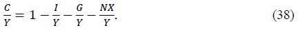
Second, the Laffer curve shifts downward with the aging population as in Trabandt and Uhlig (2011), and Auray et al. (2016) with more catching up with the Joneses households. Since households work more hours to catch up with the Joneses, pushing downward the wage rate, it is less likely to expect an increase of maximum tax revenues in the small open economy with a high degree of external habit.
Third, the tax revenues under an extreme progressive taxation regime are much lower than the revenues under a uniform taxation regime. For example, the maximum revenues associated with taxations only on labor income of asset holders are 10-20 percent less than the revenues associated with taxations on both asset holders and non-asset holders.
Finally, the less progressive the redistribution is, the larger the multiplier effect of government expenditure associated with a revenue-neutral redistribution policy is in the small open economy with both a unitary intertemporal elasticity of substitution and a unitary intratemporal elasticity between home and foreign goods as in Galí and Monacelli (2005).
The paper is structured as follows. Section II specifies a canonical two agent small open economy and derives an equilibrium. Section III and IV discuss the implications of the model related to taxes and tax revenues, i.e. the Laffer curve, and the effect of a terms of trade on the Laffer curve. Section V presents the dynamic effect of the government expenditure rise on the economy under the assumption of revenue-neutral redistribution policy in the short run. Section VI concludes the paper.
1)
2)The demographically induced effects of aging society on net exports is ambiguous depending on the relative shrink speed of saving and investment. For example, if the investment ratio (relative to the GDP) falls faster than the savings ratio due to the aging as in Japan, the current account deficits will be smaller or the current account surplus will occur.
3)Contrary to the representative agent model, there occur trade imbalances, irrespective of the intertemporal elasticity of substitution and the intratemporal elasticity of substitution between home and foreign goods in two agent model with constrained households. The degree of current account imbalances critically depends on the redistribution policy between unconstrained and constrained households, complicating the analysis of the effects of aging society on net exports.
II. The Model
This section sets up a two agent small open economy with asset holders and non-asset holders. The world is composed of two countries, home (
A share of 1 −
2.1. Households
2.1.1. Asset Holders
Asset holders maximize their life-time utility function by choosing consumption, asset holdings, and labor supply subject to a sequence of budget constraints, given by (7). The welfare of asset holder is given by

Here β is the household's discount factor and
The CD preference has a simple functional form where a closed-form solution for the equilibrium labor can be found:

Since α governs marginal rate of substitution between consumption and leisure, the higher value of 1 − α puts higher weight on leisure and induces to decrease labor supply. Hence, α can be used to calibrate the decreased labor hours in aged economy. Though the CD preference can suggest some benchmark results about the effect of the aging trend on tax revenues, it is not satisfactory since only one parameter can be used to calibrate the aging society. Because of this problem, we will present main results employing the CFE preference and leave the results associated with the CD preference in the appendix. In the CFE preference, both the intertemporal elasticity of substitution and the Frisch labor supply elasticity can be adjusted to calibrate the aging society. The CFE utility function is given by
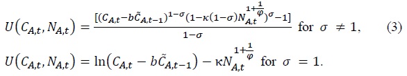
Here σ-1 and φ represent the intertemporal elasticity of substitution and the Frisch labor supply elasticity, respectively. Since  is specified as an external habit depending on only aggregate consumption as in Abel (1990), Jung (2015), and Smets and Wouters (2007). In equilibrium, it holds that
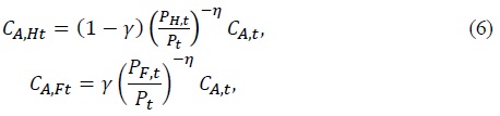
Next,
where
where
Under the small open economy assumption of
where
For the analytical simplicity, assume that domestic asset holders can trade state-contingent bonds denominated in domestic currency at the international financial market. Then, domestic asset holder’s budget constraint can be written as
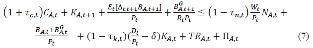
where  is one-period discount government debt which can be purchased or sold at the price of
  Here
Here
In the case of CFE preference, the optimization conditions with respect to consumption, labor hours and asset holdings are given by

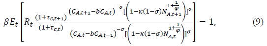
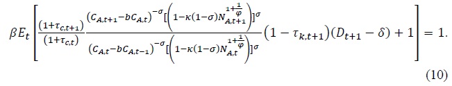
Equation (8) characterizes the labor supply decision. Equation (9) is the Euler equation and equation (10) determines the equilibrium rate of return for capital. The equilibrium real exchange rate
For the CFE preference,
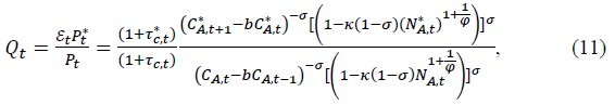
and for the CD preference,
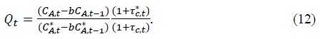
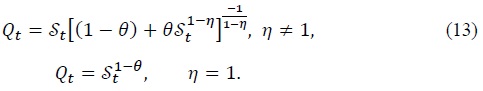
Here  and the real exchange rate are related as follows
2.1.2. Non-Asset Holders
Non-asset holders who cannot have access to financial markets just supply labor

where
Non-asset holders choose their consumption and labor supply to maximize their temporal utility function (
The optimization conditions in the CFE preference case are given by
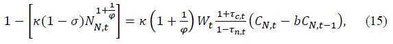
and the budget constraint (14).
2.2. Domestic firms4
Monopolistically competitive firms produce their products with a Cobb-Douglas production function:

where the productivity shock  Since labor and capital markets are perfectly competitive, the firm
Here
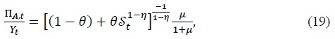
where Π
2.3. Aggregation
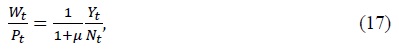
The aggregate level of any household-specific variable 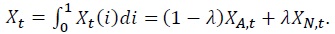 Hence, aggregate consumption and aggregate hours are given by


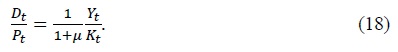
Aggregate dividend, capital, and bond holdings also satisfy


The redistribution policy satisfies the following relationship

2.4. Government
Since the government collects tax revenue ( its budget constraint can be expressed as


In (26), it is assumed that government purchases only domestic goods which is typical assumption in the small open economy literature (De Paoli, 2009; Monacelli and Perotti, 2011). We can interpret taxations on only labor income of asset holders as an extreme progressive taxation scheme. Under the extreme progressive taxation regime, the budget constraint (27) is replaced by

2.5. Equilibrium
Goods market clearing condition can be written as

where
The competitive equilibrium conditions consist of the efficiency conditions and the budget constraints of the households and firms, and the market clearing conditions of each goods market, labor market, capital, and bond market. That is, the symmetric equilibrium is a sequential allocation of  a sequence of prices and costate variables for the home country
  and a sequence of the real exchange rate
  such that (1) the asset holders and non-asset holders’ decision rules solve their optimization problems, given the states and the prices; (2) the demands for labor and capital solve each firm's profit maximization problem, given the states and the prices; (3) each goods market, labor market, capital market, and bond market are cleared at the corresponding prices, given the sequence of the variables of the reset of the world, the initial conditions for the state variables, and the exogenous shock processes as well as the monetary policy and fiscal rate
We will consider the effect of long-run fiscal policy focusing on the steady-state balanced growth equilibrium where all endogenous variables except labor hours, interest rate, tax rate grow at the same constant rate in the steady-state.
2.6. Steady-state
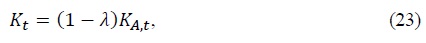
In the balanced steady-state, the ratio of consumption, capital, and investment relative to output is determined by some deep parameters and capital tax rate.
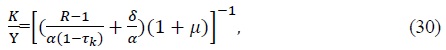
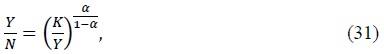
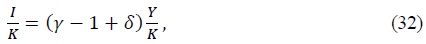


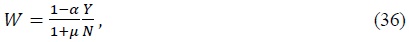
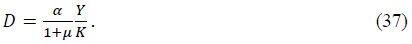
Given the values of the deep parameters such as the real interest rate, capital depreciation rate, net markup, and capital income ratio and tax rates, we can get great ratios such as  from (30)-(37). Also notice that consumption of asset holders is financed from capital and labor income,
4)The perfect pass-through is assumed so that the law of one price holds in the importing firms.
III. Laffer Curve in Neoclassical Model without Exchange Rate Channel
We consider the Neoclassical growth model à la Trabandt and Uhlig (2011) by setting the steady-state real exchange rate and terms of trade to 1 in equation (33) - (35). That is, the goods market clearing condition under the neoclassical growth model can be simplified as
In this section, we will discuss the implication of the Laffer curve in the neoclassical growth economy model without any exchange rate channel, employing (38) and CFE preference (3).
3.1. Calibration
Assuming that each agent works for 14 hours as in Park (2012) who calibrates it from the OECD, the key parameter on working hours can be calculated from the labor force data as

Since members in both asset holders and non-asset holders work for 14 hours, the average working hours can increase or decrease with the number of each cohort to work and the average working hours per worker. Hence, the participation rate in the labor market declines with the aging trend, since the average working hours per worker are the same in both the current and future state.
The Laffer curve in the steady-state can be expressed as
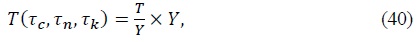
where 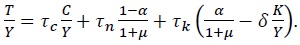
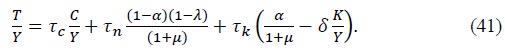
Equation (40) shows that the increase in net markup depresses the tax revenues as it shifts down the demand for goods and the aggregate output, which lowers labor-output ratio as well as the capital-output ratio. That is, the stronger the market power of firms are, the lower the revenues attributable to taxes are. If government levies taxes only on asset holders, then the Laffer curve of (40) is modified as follows:
All common parameter values used in this paper are reported in Table 1 which are taken from Galí and Monacelli (2005) and Jung (2015). First, we set both the intertemporal elasticity of substitution, σ⁻¹ and the Frisch labor supply elasticity of labor supply ν⁻¹ to 1. The intratemporal elasticity between home and foreign goods η and the degree of openness
We set the subjective discount factor to 1.04-0.4, which is consistent with an annual real rate of interest of 4 percent. Next, we set the elasticity of substitution among varieties ε to 6, implying the average size of markup, μ to be 1.2 as in Galí and Monacelli (2005). The fraction of the constrained households, λ is set to 0.3, the estimated value in Jung and Kim (2019).
Table 2 presents parameter values specific to Korea and U.S. which are taken from Park (2012) and Hur and Lee (2017). The parameter related to labor supply κ is set to 3.52, estimated value in Hur and Lee (2017), while net exports and government spending relative to GDP are set to 0.0273 and 0.1891 which are the estimated average values from 2000-2015. The capital, labor, and consumption tax rate (
In the subsequent section, we will present the quantitative result based on the CFE preference, leaving the result associated with the CD to the appendix.
3.2. Catching up with Joneses and Laffer Curve
The households with high degree of external habit persistence work more hours and consume more goods to catch up the Joneses as in Figure 1. Since households with high degree of external habit persistence are already working hours more than necessary, the expected total tax revenue by raising higher taxes on the households with external habit is lower than by raising higher taxes on the households without external habit.
The fiscal space in the paper is defined as the distance between the current revenue and the maximum revenue calculated from the Laffer curve (40). Abstracting from government’s indebtedness, it focuses only on how much the government can raise additional revenues. The
First, Figure 2A presents total tax revenue by varying the effective labor income tax rate, but fixing the capital income tax rate at the current value. The Figure shows that the total tax revenue increases up to 152 percent of the current revenue by raising the labor income tax rate to 62 percent when households do not have any degree of external habit. The aging trend shifts down the Laffer curve, making the fiscal deficit larger at any tax rate, given that the government expenditure does not change at all. The maximum total tax revenue increases up to 129 percent, much smaller than the maximum tax revenue associated with the current state to the corresponding labor income tax rate hike.
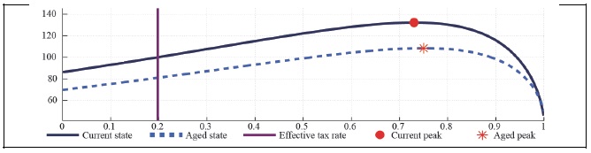
Figure 3A presents that the total tax revenue can increase up to 137 percent of the current revenue by raising the labor income tax rate to 56 percent when households have substantial degree of external habit persistence. Notice that the aging vertically shifts down the Laffer curve, irrespective of the habit persistence. The expected total tax revenue from raising the labor income tax rate in the aging economy with external habit persistence is less than the one in the aging economy without any external habit. The expected total tax revenue increases to 116 percent in the aged state to the corresponding labor income tax rate hike.
Figure 2B and 3B present total tax revenue by varying the capital income tax rate, and fixing the labor income tax rate at the current tax rate. The total tax revenues from higher capital income tax rates are a little bit smaller in the aging economy with external habit than in the aging economy without any habit, since both labor and capital are complementary in the production process as in Figure 2B and 3B.
3.2. Markup and Laffer Curve
Firms with higher markup have stronger market power and they can make higher profit per output by setting higher prices than the marginal cost. The higher the markup, the lower output. The actual output associated with the monopolistically competitive economy is much lower than the efficient natural output. Therefore, households work less hours in the economy with a higher average markup as in Figure 4. Furthermore, both the consumption and income inequality between asset holders and non-asset holders amplify with the share of non-asset holders (
Figure 6A and 6B present total labor and capital income tax revenue in the economy with a substantial degree of external habit. The expected maximum total labor and capital income tax revenue in the economy without any market power and external habit is 5 percent lower than the maximum tax revenue in the economy with substantial market power and external habit. Furthermore, the expected maximum tax revenue in the aged state is higher in the monopolistically competitive economy than in the perfectly competitive economy, since households work more hours to compensate for the loss of disposable income.
3.3. Progressive Labor Income Tax: Tax exempt to Non-asset holders
In this subsection, we consider the effect of progressive taxation on the total tax revenue. Campbell and Mankiw (1989) and Kaplan et al. (2016) show that one third of the U.S. households consume their period-labor income every period, i.e. consumption of 30-40 percent U.S. households tracks the current income. The tax exempt to non-asset holders has a feature of redistribution policy from asset holders to non-asset holders.
Figure 7-Figure 9 present the effect of taxes on asset holders with tax exempt to non-asset holders in the economy with a fraction of non-asset holders equal to 0.3. In the two agent economy, the progressive tax scheme with tax exempt to non-asset holders lowers the expected maximum labor tax revenue up to 20 percent, irrespective of the market structure and catching up with the Joneses. The progressive taxation also shifts down the Laffer curve vertically in the aged state, resulting in a larger fiscal deficit, unless government does not cut the aging-related expenditure.
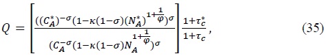
IV. Laffer Curve in a Small Open Economy with Exchange Rate Channel
In this section, we will also consider the effect of higher tax rates on total tax revenues, taking into account the effect of consumption tax on the real exchange rate by setting
If the intertemporal elasticity of substitution is different from one, both consumption and labor hours matter to the equilibrium real exchange rate, complicating the solution of consumption and labor hours in the steady-state. For the sake of analytical simplicity, we assume that the intertemporal elasticity of substitution equals one and consumption of domestic asset holders equals foreign household’s consumption.
4.1. Catching up with the Joneses and Laffer Curve
Figure 10A and 11A present the capital and labor Laffer curve in the small open economy with perfect competition and CFE preference taking into account the effect of consumption tax on the real exchange rate. The higher the domestic consumption tax rate relative to the foreign tax rate is, the lower the real exchange rate is, and the higher the purchasing power of domestic households is. Comparison of Figure 2A and Figure 10 A shows that the expected maximum total tax revenue by raising taxes on labor and capital is marginally smaller in the small open economy with the exchange rate channel than in the economy without any exchange rate channel. The expected maximum total tax revenue in the aged state is also marginally smaller in the economy with the real exchange rate channel than the one in the neoclassical economy, since the expenditure switching effect associated with the terms of trade variation diverts the demand for goods toward foreign goods, contracting domestic production.
If households do not have any habit persistence, then the maximum labor tax revenue amounts to 151 percent in the current state while it drops to 128 percent in the aged state. The expected maximum labor tax revenue in the economy with external habit is not much different from the one in the economy without any habit. The maximum labor tax revenue in the current state reaches to 151 percent, while it drops to 127 percent in the aged state. Next, consider the effect of capital tax rate on total tax revenue. Figure 10B and 11B present the capital Laffer curve, showing similar features as the labor Laffer curve. The capital Laffer curve marginally shifts downward with the real exchange rate appreciation as the labor Laffer curve. Comparison of Figure 2 and Figure 10 shows that the effect of asymmetric consumption taxations (
4.2. Markup and Laffer curve
Figure 12 and 13 present the tax revenue when households have a CFE preference in the monopolistically competitive economy, taking into account the effect of consumption tax on the real exchange rate. The effect of consumption tax rate on the capital and labor Laffer curve also matters little in the monopolistically competitive economy.
Comparison of Figure 10 and Figure 12 show that there is a marginal difference between the Laffer curve associated with the perfectly competitive economy and the one with monopolistically competitive economy, whether we take into account the exchange rate channel on the economy or not as in previous section. The features associated with the perfectly competitive economy holds in the monopolistically competitive economy, whether households have external habit or not as in Figure 12 and 13.
4.3. Progressive Labor Income Tax: Tax exempt to non-asset holders
Figure 14-15 present how the progressive taxations, i.e. taxations only on asset holders affect the labor and capital Laffer curve in the monopolistically competitive economy when households have external habit persistence in consumption. Comparison of Figure 5 and Figure 14 shows that the progressive taxations with the tax exempt to non-asset holders and higher burden to asset holders decreases about 20 percent of the maximum capital and labor tax revenues.
The taxation on asset holders and tax exempt to non-asset holders make the labor and capital Laffer curve to shrink whether the economy is in the aged state or not. The progressive taxation entails a trade-off between the moderation of consumption inequality and the available tax revenues.
V. Fiscal Policy and Redistribution
In previous section, we have discussed the capital and labor Laffer curve in the long run under the assumption of either a uniform taxation or an extreme redistribution policy in place, i.e. the form of tax exempt to non-asset holders. In this section, we will address the dynamic effect of government spending rise on the economy under alternative redistribution policy as in Debortoli and Galí (2017).
To look at the short run effect of redistribution policy on the economy, we consider a within period balanced transfer to non-asset holders by taxes on asset holders. By construction, this revenue-neutral tax cut policy which changes the life-time income of households has a property of intratemporal redistribution. Suppose that non-asset holders receive some transfers from the asset holders as follows

Here

If
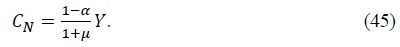
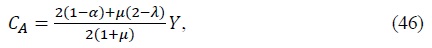
First, consider the laissez-faire regime. The steady-state consumption of asset holders and non-asset holders is given by
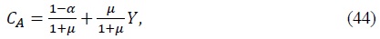
Hence, the consumption inequality between asset holders and non-asset holders is given by 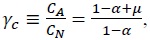 implying that the higher markup increases profits per output, which deteriorates the consumption inequality between asset holders and non-asset holders.
Next, consider the revenue-neutral uniform redistribution policy (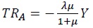 to each asset holder and redistributes
 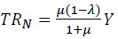 to each non-asset holder, inducing both asset holder and non-asset holder to consume the same amount of goods at the steady-state.
Finally, consider the more practical scenario by assuming revenue-neutral partial income redistribution policy. Suppose that government taxes half of the dividend income to each asset-holder and then redistribute it to each non-asset holder. That is, 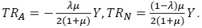 Then, the steady-state consumption of asset holder and non-asset holder is given by

Under the partial redistribution policy, the consumption inequality between asset holder and non-asset holder equals 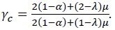
Figure 16 and Figure 17 present the effect of expansionary fiscal policy under a uniform redistribution policy every period (
Under a uniform redistribution policy regime, both asset holders and non-asset holders receive the same amount of dividend income from firms. Hence, non-asset holders reduce their labor hours, but they can consume more goods to the favorable government spending shock. However, asset holders should work more hours and reduce their consumption to smooth out the tax burden over time. The government spending multiplier associated with a uniform redistribution regime in the two agent economy is similar to the one of the representative agent economy, since there occurs a crowding effect.
Under a partial redistribution regime, the less partial the redistribution policy is, the stronger the effect of government spending is as in Figure 19. That is, the more progressive the redistribution policy is, the stronger the crowding effect of the government spending is. The government spending multiplier can be larger than one under a weak partial redistribution regime, since the government spending rise increases not only investment but also non-asset holder’s consumption with a mild fall of asset holder’s consumption. The fiscal multiplier is largest under the laissez-faire regime, since asset holder’s consumption changes a little, which entails a mild variation of the terms of trade. There occurs a very mild negative effect of the terms of trade on domestic production.
VI. Conclusion
This paper sets up a two agent small open economy with monopolistically competitive firms and aging population by extending the neoclassical growth model of Trabandt and Uhlig (2011) and then investigates the labor and capital Laffer curve. The paper also looks at the effect of tax rate on the Laffer curve, taking into account the change of the real exchange rate associated with the consumption taxes along the line Galí and Monacelli (2005) and Auray et al. (2016)
The paper finds that the higher the market power of firms is, the larger the consumption inequality between asset holders and non-asset holders is. Hence, there is room for government to increase the tax revenue by raising tax rates under the economy with higher markup, since households will work more hours to compensate for their loss of labor income to tax hikes. However, the expected maximum tax revenue is likely to shrink with the degree of external habit in consumption, since households with external habit have worked more hours than necessary to catch up with the Joneses, shifting up less in the aged state.
The paper also finds that there occurs a substantial decrease in the labor and capital tax revenue if government raises taxes only to asset holders with non-asset holders exempt. Finally, it finds that the fiscal multiplier shrinks with the degree of progressive redistribution policy.
Tables & Figures
Table 1.
Common Parameter Values
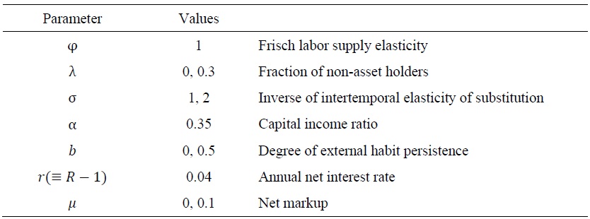
Table 2.
Country Specific Parameter Values
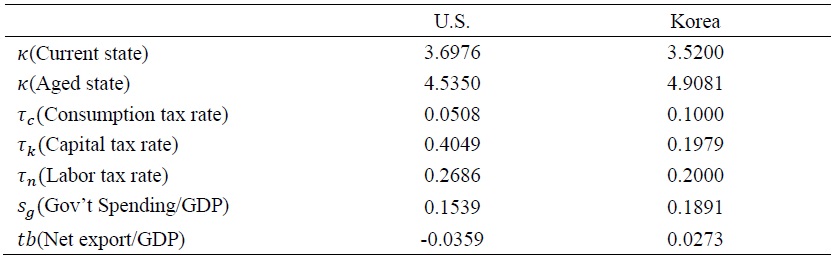
Note: Current state: 2010; Aged state: 2050.
Sources:
Figure 1.
Degree of Habit and Labor Hours
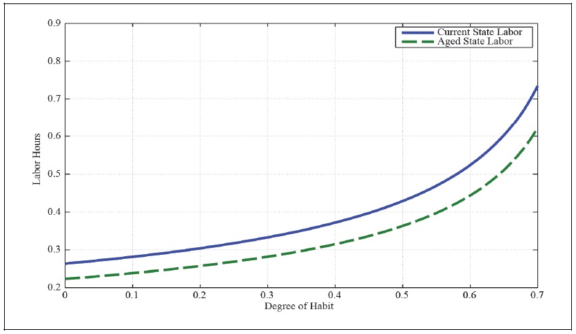
Figure 2A.
Labor Laffer Curve with CFE Preference (b = 0,
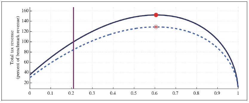
Figure 2B.
Capital Laffer Curve with CFE Preference (b = 0,
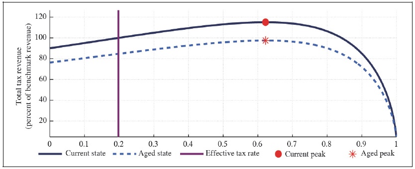
Figure 3A.
Labor Laffer Curve with CFE Preference (b = 0.5,
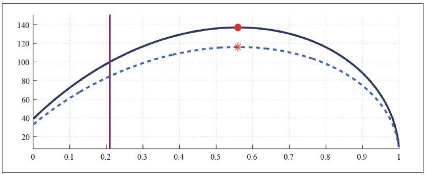
Figure 3B.
Capital Laffer Curve with CFE Preference (b = 0.5,
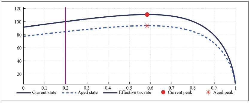
Figure 4.
Degree of Markup and Labor Hours
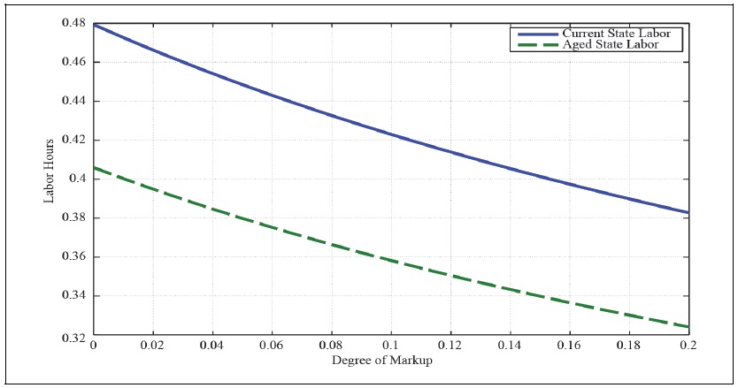
Figure 5A.
Labor Laffer Curve with CFE Preference (b = 0,
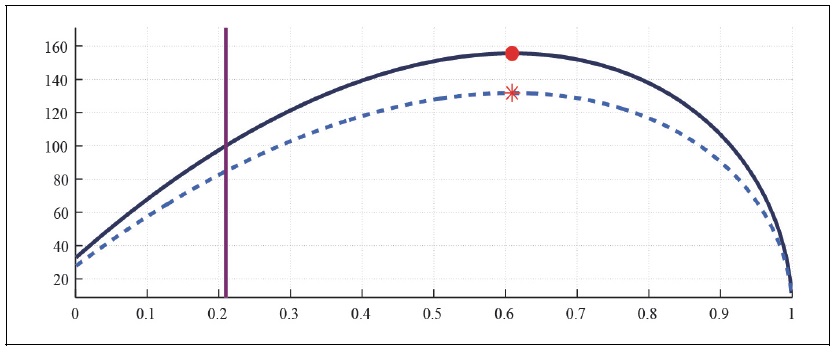
Figure 5B.
Capital Laffer Curve with CFE Preference (b = 0,
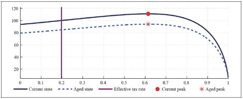
Figure 6A.
Labor Laffer Curve with CFE Preference (b = 0.5,
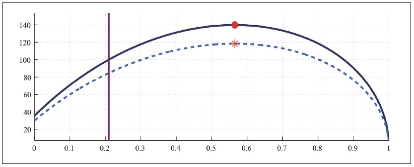
Figure 6B.
Capital Laffer Curve with CFE Preference (b = 0.5,
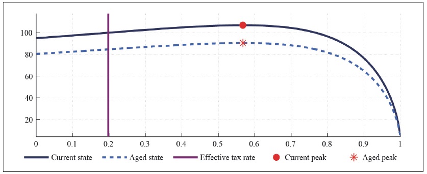
Figure 7A.
Labor Laffer Curve with CFE Preference (b = 0,
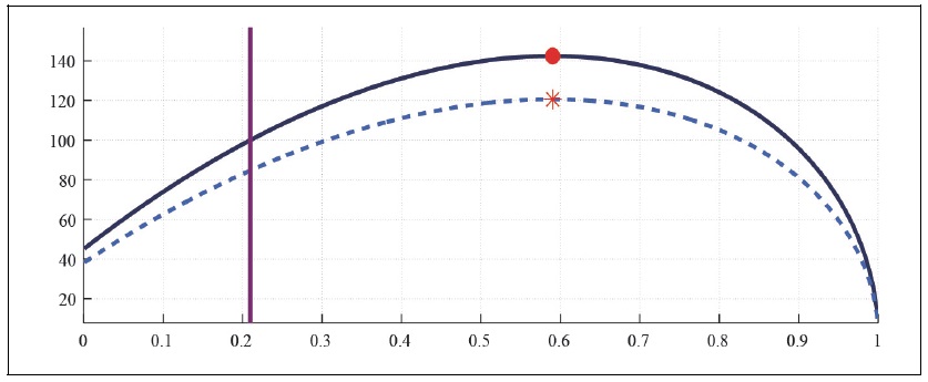
Figure 7B.
Capital Laffer Curve with CFE Preference (b = 0,
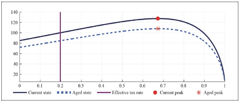
Figure 8A.
Labor Laffer Curve with CFE Preference (b = 0.5,
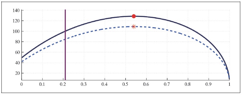
Figure 8B.
Capital Laffer Curve with CFE Preference (b = 0.5,
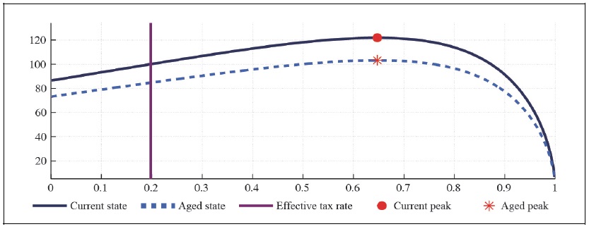
Figure 9A.
Labor Laffer Curve with CFE Preference (b = 0.5,
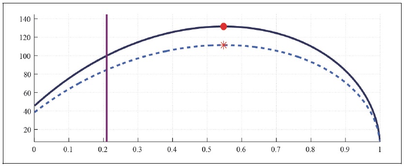
Figure 9B.
Capital Laffer Curve with CFE Preference (b = 0.5,
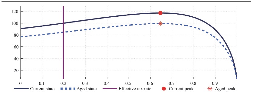
Figure 10A.
Labor Laffer Curve with CFE Preference (b = 0, S = 0.927,
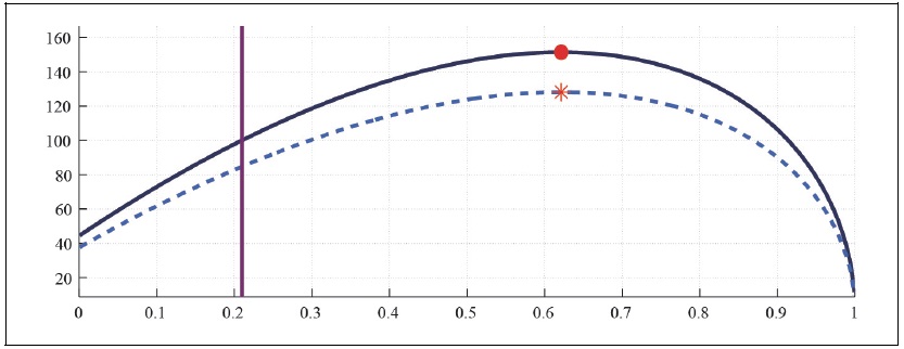
Figure 10B.
Capital Laffer Curve with CFE Preference (b = 0, S = 0.927,
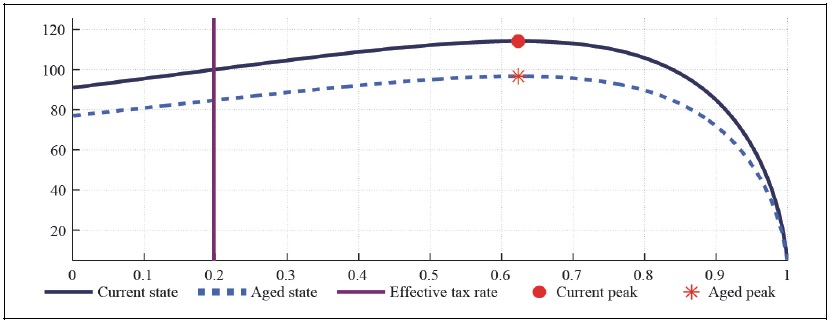
Figure 11A.
Labor Laffer Curve with CFE Preference (b = 0.5, S = 0.927,
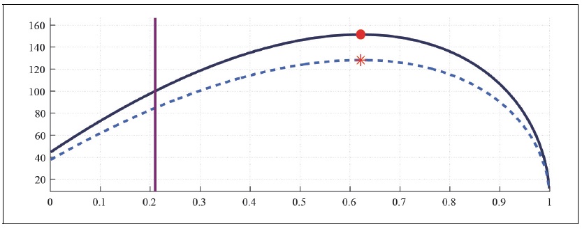
Figure 11B.
Capital Laffer Curve with CFE Preference (b = 0.5, S=0.927,
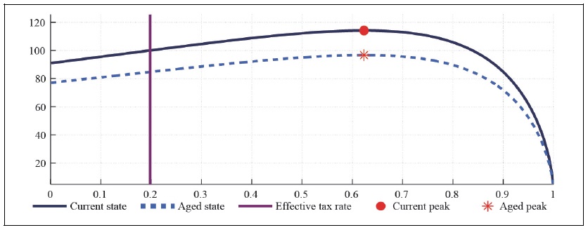
Figure 12A.
Labor Laffer Curve with CFE Preference (b = 0, S = 0.927,
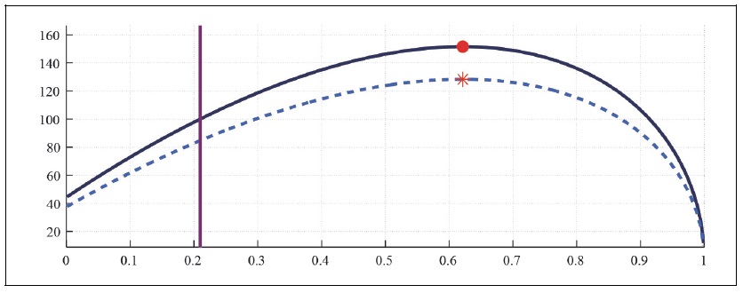
Figure 12B.
Capital Laffer Curve with CFE Preference (b = 0, S = 0.927,
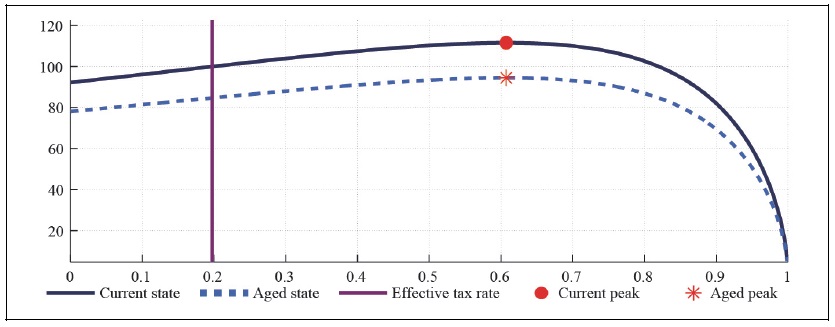
Figure 13A.
Labor Laffer Curve with CFE Preference (b = 0.5, S = 0.927,
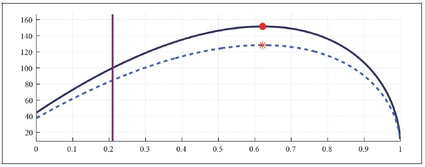
Figure 13B.
Capital Laffer Curve with CFE Preference (b = 0.5, S = 0.927,
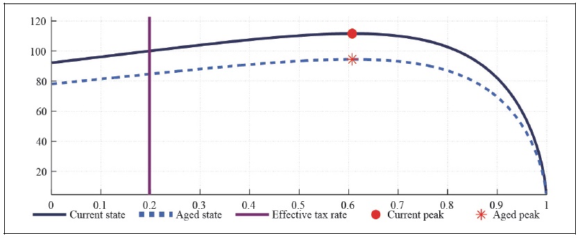
Figure 14A.
Labor Laffer Curve with CFE Preference (b = 0, S = 0.927,
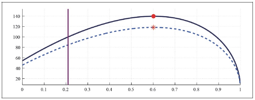
Figure 14B.
Capital Laffer Curve with CFE Preference (b = 0, S = 0.927,
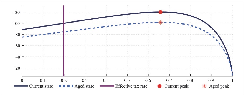
Figure 15A.
Labor Laffer Curve with CFE Preference (b = 0.5, S = 0.927,
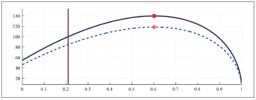
Figure 15B.
Capital Laffer Curve with CFE Preference (b = 0.5, S = 0.927,
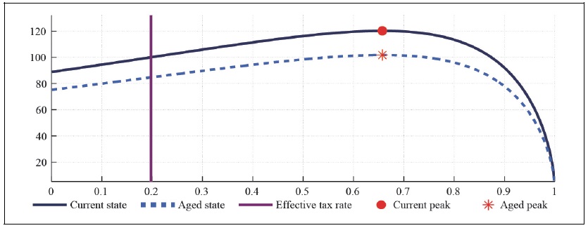
Figure 16.
Impluse Respsonse Function to a Positive Goverment Spending Shock with Redistribution (
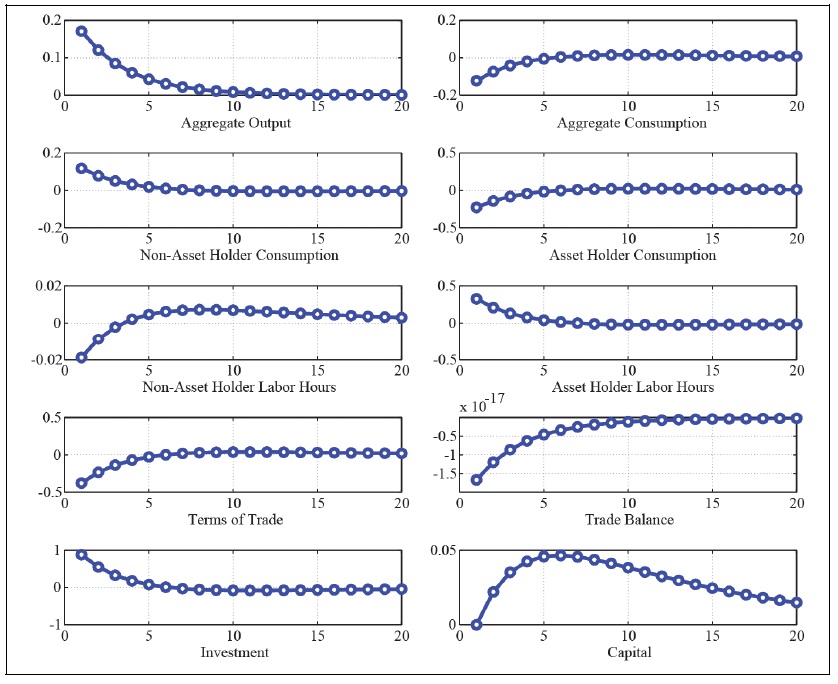
Figure 17.
Impluse Respsonse Function to a Positive Goverment Spending Shock with Redistribution (
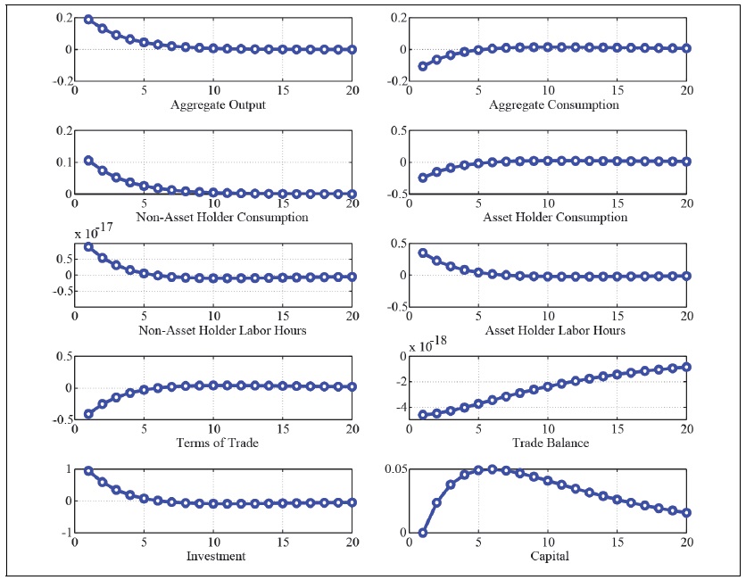
Figure 18.
Impluse Respsonse Function to a Positive Goverment Spending Shock with Redistribution (
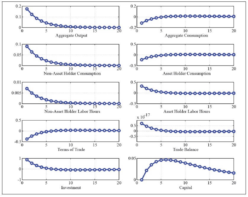
Figure 19.
Impluse Respsonse Function to a Positive Goverment Spending Shock with Redistribution (
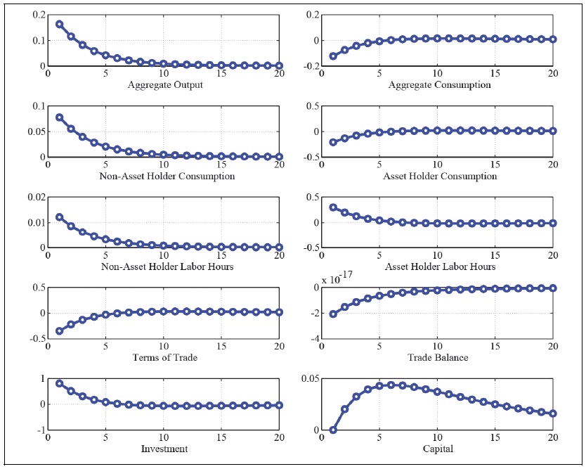
Figure 20A.
Labor Laffer Curve with CD Preference (b = 0,
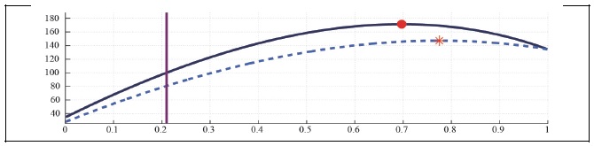
Figure 20B.
Capital Laffer Curve with CD Preference (b = 0,
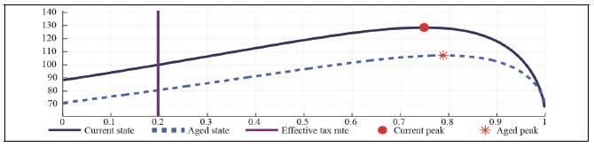
Figure 21A.
Labor Laffer Curve with CD Preference (b = 0.5,
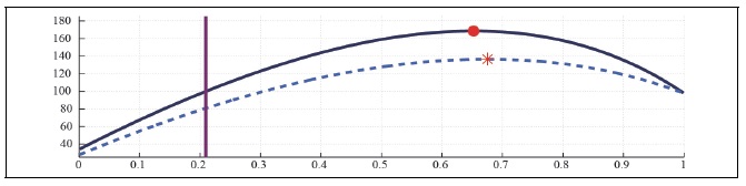
Figure 21B.
Capital Laffer Curve with CD Preference (b = 0.5,
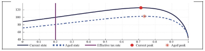
Figure 22A.
Labor Laffer Curve with CD Preference (b = 0,

Figure 22B.
Capital Laffer Curve with CD Preference (b = 0,
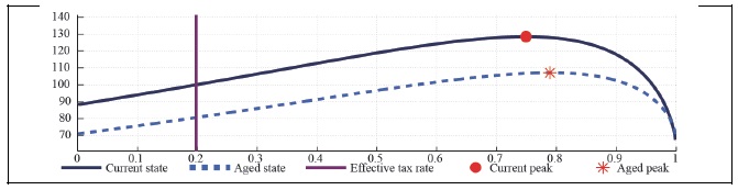
Figure 23A.
Labor Laffer Curve with CD Preference (b = 0.5,
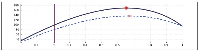
Figure 23B.
Capital Laffer Curve with CD Preference (b = 0.5,
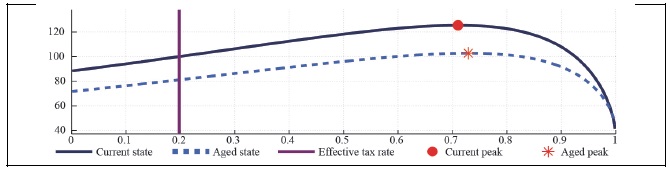
Figure 24A.
Labor Laffer Curve with CD Preference (b = 0, S = 0.927,
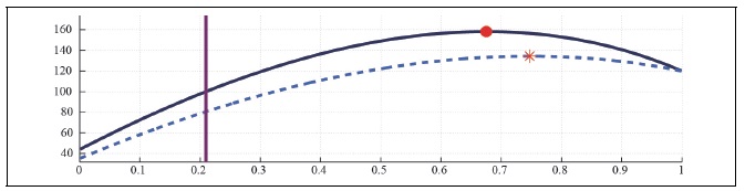
Figure 24B.
Capital Laffer Curve with CD Preference (b = 0, S = 0.927,
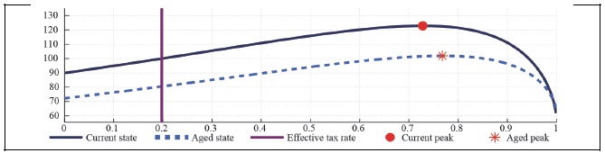
Figure 25A.
Labor Laffer Curve with CD Preference (b = 0.5, S = 0.927,
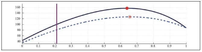
Figure 25B.
Capital Laffer Curve with CD Preference (b = 0.5, S = 0.927,
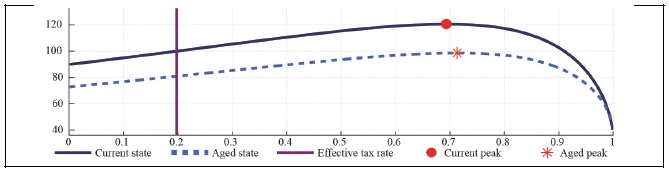
Figure 26A.
Labor Laffer Curve with CD Preference (b = 0, S = 0.927,
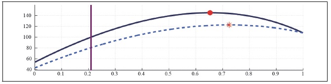
Figure 26B.
Capital Laffer Curve with CD Preference (b = 0, S = 0.927,
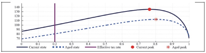
Figure 27A.
Labor Laffer Curve with CD Preference (b = 0.5, S = 0.927,
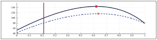
Figure 27B.
Capital Laffer Curve with CD Preference (b = 0.5, S = 0.927,
References
- Abel, A. B. 1990. “Asset Prices under Habit Formation and Catching Up with the Joneses.” Papers and Proceedings of the Hundred and Second Annual Meeting of the American Economic Review, vol. 80, no. 2, pp. 38-42.
-
Auray, S., Eyquem, A. and P. Gomme. 2016. “A Tale of Tax Policies in Open Economies.”
International Economic Review , vol. 57, no. 4, pp. 1299-1333.
-
Bilbiie, F. O. 2008. “Limited Asset Market Participation, Monetary Policy, and (Inverted) Aggregate Demand Logic.”
Journal of Economic Theory , vol. 140, no. 1, pp. 162-196.
-
Bilbiie, F. O., Monacelli, T. and R. Perotti. 2013. “Public Debt and Redistribution with Borrowing Constraints.”
Economic Journal , vol. 123, no. 566, pp. F64-F98.
-
Campbell, J. Y. and N. G. Mankiw. 1989. “Chapter 4: Consumption, Income and Interest Rates: Reinterpreting the Time Series Evidence.” In Blanchard, O. J. and S. Fisher. (eds.)
NBER Macroeconomics Annual 1989 , Volume 4. Cambridge, MA: MIT Press. pp. 185-246. - Debortoli, D. and J. Galí. 2017. Monetary Policy with Heterogeneous Agents: Insights from TANK Models. [Preliminary and Incomplete] CREi Working Papers. Centre de Recerca en Economia Internacional.
-
De Paoli, B. 2009. “Monetary Policy and Welfare in a Small Open Economy.”
Journal of International Economics , vol. 77, no. 1, pp. 11-22.
-
Galí, J. and T. Monacelli. 2005. “Monetary Policy and Exchange Rate Volatility in a Small Open Economy.”
Review of Economic Studies , vol. 72, no. 3, pp. 707-734.
-
Gonzalez-Eiras, M. and D. Niepelt. 2012. “Aging, Government Budgets, Retirement, and Growth.”
European Economic Review , vol. 56, no. 1, pp. 97-115.
-
Hur, J. and K. K. Lee. 2017. “Fiscal Financing and the Efficacy of Fiscal Policy in Korea: An Empirical Assessment with Comparison to the U.S. Evidence.”
Economic Modelling , vol. 64, pp. 473-486.
-
Jung, Y. 2015. “Price Stability in Economies with Habit Persistence.”
Journal of Money, Credit and Banking , vol. 47, no. 4, pp. 517-549.
-
Jung, Y. and Y. Kim. 2019. “Liquidity Constraint, Consumption Volatility and Consumption Gap.”
Journal of Korean Economic Analysis , vol. 25, no. 2, pp. 99-156. (in Korean) - Kaplan, G, Moll, B. and G. L. Violante. 2016. Monetary Policy According to HANK. NBER Working Paper, no. 21897. National Bureau of Economic Research.
-
Monacelli, T. and R. Perotti. 2011. “Redistribution and the Multiplier.”
IMF Economic Review , vol. 59, no. 4, pp.630-651.
- Ostry, J. D., Ghosh, A. R., Kim, J. I. and M. S. Qureshi. 2010. Fiscal Space. IMF Staff Position Note, no. SPN/10/11. International Monetary Fund.
- Park, S. G. 2012. Quantifying Impact of Aging Population on Fiscal Space. IMF Working Papers, no. 12/164. International Monetary Fund.
- Song, H. and J. Hur. 2017. Impact of Ageing on the Public Finance. BOK Working Paper, no. 2017-29. Bank of Korea. (in Korean)
-
Smet, F and R. Wouters. 2007. “Shocks and Frictions in US Business Cycles: A Bayesian DSGE Approach.”
American Economic Association , vol. 97, no. 3, pp. 586-606. -
Trabandt, M. and H. Uhlig. 2011. “The Laffer Curve Revisited.”
Journal of Monetary Economics , vol. 58, no. 4, pp. 305-327.