

- EAER>
- Journal Archive>
- Contents>
- articleView
Contents
Citation
| No | Title |
|---|
Article View
East Asian Economic Review Vol. 25, No. 4, 2021. pp. 403-424.
DOI https://dx.doi.org/10.11644/KIEP.EAER.2021.25.4.402
Number of citation : 0View
52
Download
30
Forecasting KOSPI Return Using a Modified Stochastic AdaBoosting
|
|
Sungkyunkwan University |
|---|---|
|
|
Yonsei University-Mirae Campus |

Abstract
AdaBoost tweaks the sample weight for each training set used in the iterative process, however, it is demonstrated that it provides more correlated errors as the boosting iteration proceeds if models’ accuracy is high enough. Therefore, in this study, we propose a novel way to improve the performance of the existing AdaBoost algorithm by employing heterogeneous models and a stochastic twist. By employing the heterogeneous ensemble, it ensures different models that have a different initial assumption about the data are used to improve on diversity. Also, by using a stochastic algorithm with a decaying convergence rate, the model is designed to balance out the trade-off between model prediction performance and model convergence. The result showed that the stochastic algorithm with decaying convergence rate’s did have a improving effect and outperformed other existing boosting techniques.
JEL Classification: C32, C50, G12
Keywords
Machine Learning, AdaBoost, XGBoost, Decaying Convergence Rate
I. Introduction
As the interest in the field of machine learning intensifies, the ensemble learning scheme has drawn much attention. The model ensemble includes all the schemes that try to combine several different models to produce a committee’s decision, in the sense that a mixture of models produces better results than a single model. From the human’s point of view, it is similar to listening to the many experts. There are various methodologies to combine the models. Bootstrap aggregating chooses to combine several different classifiers that are trained with different bootstrapped training data at the same time. To put it in the same analogy, it is asking for the voter’s opinion where voters have bits and pieces of information. On the other hand, boosting takes an additive approach, where a classifier’s training information is passed on to the next iteration phase. Using the same analogy, it is the same as asking for the voter’s opinion one by one, during which the next voter gets the result of the previous voter. Because the ensemble scheme uses several models at once, the major advantage of boosting is that the researcher is free of investigating the best model that fits in every situation.
It is natural to assume that each voter we ask would make their choices independently, in other words, the voters would choose their prediction result independently from others. It is known that the importance of diversity is more important than the quality of the individual voting component itself (Hsu, 2017). However, the original AdaBoost does not consider the correlation between the classifier’s results. Also, some variants of AdaBoost, such as that of Li et al. (2008) uses only one type of model to make a combined result. Machine learning models see data from a different perspective. Support vector machine tries to find the best hyperplane that separates the data. The best hyperplane is attained by choosing the hyperplane that provides the most gap between the plane and the closest vectors to the plane (Boser et al., 1992). However, a classifying neural network is fitted by using multiple steps of non-linear transformation. In this sense, the support vector and neural network see the data in different ways, and naturally, their difference in model structure would produce an independent prediction. Therefore, it is reasonable to assume that including more models in the voter set will be beneficial.
There are myriads of researches regarding predicting economic variables such as daily stock market direction. In the recent rise of the interest in the field of machine learning techniques, most of the researches focus on improving the benchmark scores using different kind of preprocessed or unprocessed data. A study done by Zhong and Enke (2019) used a hybrid machine-learning algorithm to predict the daily return direction of S&P 500 ETF using 60 economically related features. They tested variously configured deep neural networks (DNNs) model and artificial neural networks (ANNs) model using differently preprocessed dataset. The study showed that the DNN configuration that curbed the over-fitting problem by using two principal component analysis (PCA) produced the best prediction result. Furthermore, it showed that the trading strategies with the DNN classification scheme performed the best among the benchmark models.
Ng (2014) focused on boosting algorithm, which is a combination of models, rather than using single classification models to predict the target economic variable. The study aimed to sort out the relevant variable that could be potential predictors in forecasting the economic recessions in three, six, and twelve months ahead. It used over 132 financial time series variables with their lag to create over 1500 variables. Boosting algorithm identified Aaa spread, risky bond and 5 year spread as important predictors in forecasting recessions. Also Bai and Ng (2009) used L2 boosting methodology to select predictors in factor-augmented autoregressions. The noticeable features of this research is that it implemented a stopping rule for boosting to prevent the model from being over-fitted. The study showed that one of the boosting methods outperformed conventional factor-augmented forecasting models, and autoregressive forecast.
The direct implementation of diversity tackling algorithm into boosting can be found in Li et al. (2008), which suggested boosting support vector machine with consideration of diversity inside the ensemble model. It suggested that as the classifier’s performance gets higher, the ensemble model’s diversity decreases since the individual classifiers will produce equally good results. Therefore the paper suggests artificially reducing the accuracy of the component classifiers by tempering them with the tuning parameters of the support vector machine. Also, it proposed an additional algorithm that calculates diversity during the AdaBoost algorithm. If the training error is too large, or the diversity becomes too small, the suggested algorithm adjusts the tuning parameters, keeping the diversity of the component classifiers in consideration.
Hsu (2017) proposed that the ensemble model should use multiple types of component classifiers with a heterogenous AdaBoost algorithm. To reduce the calculation overload, and add diversity to the design of the algorithm itself, he suggested an AdaBoost that chooses a single component classifier for an iteration by introducing a classifier choosing weight. The AdaBoost algorithm is part of the family of boosting algorithms that use sequentially growing decision trees as weak learners and punishing incorrectly predicted samples by assigning a larger weight to them after each round of prediction. This way, the algorithm is learning from previous mistakes, and enables us to make a final prediction by weighted majority vote. However, the algorithm itself usually is computationally very demanding and requires massive computing time as well. Moreover, for noisy data the performance of AdaBoost is controversial in the sense that it often leads to poor performance due to the algorithm spending too much time on learning process and may generate skewed results.
We believe that diversity is the most important factor that affects the overall predicting performance of the boosting algorithm. Thus, we propose a novel algorithm of AdaBoost where the heterogeneity of voting components of AdaBoost and adjusting the phase by phase sample weight change would provide more diversity into the algorithm. Following the idea of the stochastic gradient descent method that is commonly used in the field of stochastic programming, we propose a faster convergence algorithm that can be used in the procedure.
The step-size is a critical in optimization procedure of stochastic gradient descent in learning process. As is well known, too large step-size may lead non-convergence, whereas too small step size leads to slow convergence and bad local minima. As long as the iterations do not diverge, a large constant step-size promotes fast convergence. To increase the accuracy, the step-size has to be decreased. Instead of fixed step size, the decaying step-size was shown to accelerate the convergence of SGD and to yield significant improvements compared to other type of boosting procedures as shown in Huang et al. (2017) among many others.
We apply this idea in boosting algorithm in this paper. Instead of fixed sample weights and boosting iterations, we propose the exponential decaying algorithm in the adaboosting process. This leads to the faster convergence by taking big steps that can eliminate some models among the pool of classifiers with poor performance boosts by substantially decreasing the probability of being chosen. Hence, it can allow us to get faster convergence and better performances of our stochastic programming problem.
This paper is structured as follows. Chapter II will discuss the nature of the data. Finally, Chapter III and Chapter IV will cover the model used in the paper, methods to improve the original AdaBoost by inducing diversity among the voters artificially, and its fitting and prediction result.
II. Data
1. Preprocessing Liquid Market Data
To model the stock market return, we have collected various financial indicators across various fields from different sources. The collected data mostly focused on liquid markets, such as stock indices and individual stocks. Among the collected time series data, those that satisfied two conditions were eventually used in the analysis process; data should be consistently available throughout the whole examination period, and the data should represent comprehensive information regarding the market’s movement. As a result, daily data from 2014-02-02 to 2020-04-30 across 192 different indices were collected.
34 countries’ stock market indices were collected across the continent of America, Asia, and Europe using investing API. However, in concatenating the different country’s information, the time zone difference must be considered. When making an educated guess to predict market indices, one would like to use as much information as possible. Therefore, we refitted the model at 6:00 AM Korean Standard Time (KST, GMT+09) when we can use the data from the American and European Market.
Moreover, the data set include additional 10 foreign exchange rates against the United States dollar, to accommodate changes in the currency market, 64 bonds yield from 24 countries to capture the movement of alternative assets, and 8 macroeconomic variables such as LIBOR (London Inter-bank Offered Rate) rate, gold price, and crude oil prices.
Since each country has its national holidays and time zone difference, it is crucial to match the dates of each column of the data set. It is also important to fill in the blank spaces inside each column, where the stock market closes during national holidays. Therefore, we used the front-filling method, where the blank spaces are filled with the most recent data. For example, if country A’s stock market was closed on November 1st due to a national holiday, the prediction would automatically use the most recent stock market index of country A, which was recorded on October 31st. This represents the rational behavior of using every piece of information in hand at the time of prediction. After filling in the blanks, a total of 192 columns remained, which are illustrated in Table 1.
The data is transformed following the criteria suggested by FRED-MD (McCracken and Ng, 2016).
• For the interest rates such as LIBOR, TED spread and effective federal funds rate (FFR), we used first difference of original values (Δ
• For trading volume, first difference were used.
• In case of stock market indices and individual stocks from KOSPI50, log-difference were applied (Δlog
• Finally, for crude oil prices, we used second log-difference (Δ2log(
The same process was applied two more times, but with a 7-day difference and 30-day difference to take care of weekly, and monthly effects. After that, all the processed raw inputs were concatenated to form high-dimensional data set with 764 columns and 2279 rows.
For the target variable, we let
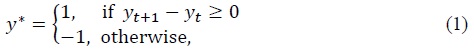
where the target variables take only two values; 1 and -1. To construct the target variable, we took the first difference of the KOSPI200 index. If the calculated difference were negative, the target variable was set to -1, and if the difference were positive, the target variable was set to 1.
2. Variable Selection
Using as much data as possible might help to find the optimization point and attain maximum training accuracy, it does not necessarily guarantee low generalization error. On the contrary, the model might be over-fitted and leads to poor out-of-sample prediction (Guyon et al., 2006). Therefore, we used permutation variable importance with random forest to choose features that have the most explanatory power.
Random forest uses differently constructed decision trees as weak classifiers to create a combined ensemble decision. Trees are trained with a different bootstrap sample of the original training set. Bootstrap samples are obtained by drawing the same number of data points with replacement. Therefore, when there are  For the whole data set, the probability of not picking
  and with large enough
First, the classification of the random forest is performed. After training, the prediction is performed using OOB samples, where each tree’s prediction value is recorded. Then the values are randomly permuted across the column, and the training is repeated. If the column possesses any prediction power, the prediction value of the original data set would exceed the data set that used the permuted one. The importance of the feature can be defined as a difference between the number of correct votes cast in the original and permuted system divided by a number of data points.
After the variable selection, 66 variables were selected among 764 original variables. Selected variables are tabulated in Table 2.
III. Model and Estimation
1. Model
Boosting aggregate the outputs of various weak classifiers to produce a powerful committee. Weak classifiers’ performance on any training set is slightly better. However, unlike bagging, where multiple weak classifiers are trained at the same time, boosting trains its classifiers in an iterative fashion. At each iteration, the training set used by the classifier is altered, as the algorithm tries to exaggerates the effect of unsuccessfully predicted observations.
(1) AdaBoost
One of the most popular boosting algorithms is an adaptive boosting algorithm or AdaBoost for short (Freund and Schapire, 1997). AdaBoost uses sample weights and updates them every iteration. The weak classifier’s performance is evaluated by the sum of that sample weights, where the word ‘adaptive’ comes from. The voting classifiers from each iterative step are aggregated via a weighted majority voting system.
Table 3 shows the AdaBoost algorithm in detail. To elaborate on each part, suppose the AdaBoost model is iterated up to
The error of individual observation takes the form of

where


where
In the next iteration,
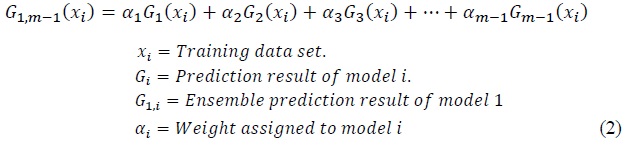
At the point of adding
To obtain the appropriate


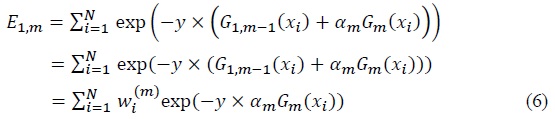
where the first element on the right hand side is the sum of all correctly classified observations and the latter element is the sum of all incorrectly classified observations. Since  is normalized into 1, the objective function becomes


where (exp(2
As for the weight of the classifier

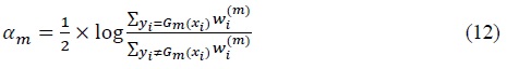

Since the voting classifier is weak, they are assumed to have a minimum accuracy of 0.5. If the
(2) XGBoost
XGBoost stands for Extreme Gradient Boosting (Chen and Guestrin, 2016). As the name suggests, it uses gradient boosting methods, and it utilizes both hardware and algorithm optimizations to maximize calculation efficiency. In algorithm optimization, XGBoost tries to improve base classifiers, which are decision trees, by employing parallel calculation, tree-pruning, and regularization. It also utilizes missing value handling techniques. By doing so, it offers many fast and efficient ways to handle large dimensional data.
XGBoost’s essence lies in its core voting classifiers: gradient boosted decision trees. Gradient boost takes a different approach compared to the AdaBoost algorithm. While in AdaBoost the errors of the models are identified by observations with relatively higher weight, in gradient boosting, they are identified by gradients. By calculating the gradients, at each iteration, the objective of the gradient boosting algorithm is to find a classifier that gives the largest improvement to the loss function
Assume that there is a loss function


where
Therefore, choosing
Just like gradient boosting, the gradient boost will also take the approach of taking the steepest descent. After determining the steepest gradient at each iteration,


In most cases, the gradient of the loss function with negative sign -∇


Since it is much faster to calculate residuals than the actual gradient in some functions, at each step, the gradient descent fits model
After the iteration phase is finished, the final boosting decision is made by updating the model at iteration in an additive manner just like AdaBoost. Table 4 illustrates the iterative process of the gradient boost algorithm.

XGBoost is based on the concept of gradient boost. While gradient boost can take any voters, XGBoost uses decision trees. XGBoost uses novel ways to shorten the model training time, and one way of doing it is to approximate the best split for each branch of the decision tree. For example, if the data has 50 features and each feature has 10 different values, one must evaluate 500 different split points. If there are more features or more values, the number of potential splitting points increases. Therefore, to reduce the split evaluating time, XGBoost creates an approximate algorithm. Essentially, it breaks down all the potential candidates for splitting points and maps it into a bucket. For example, 500 different split points can be mapped into 50 buckets, where each bucket contains 10 splitting points. Then the greedy algorithm for finding the best split is executed. By dividing it into buckets, the total number of split points to evaluate is decreased, and it can also be calculated in parallel, thereby greatly reducing the calculation time.
Furthermore, XGBoost can efficiently handle missing values in the data, by employing a sparsity-aware split finding method. XGBoost tackles the missing value problem by setting up an initial default direction for empty values, and when the algorithm encounters missing data during the inference phase, it automatically fills the missing data with the default direction. The default direction is chosen by comparing the results between two different data configurations: 1) when missing values are sent to the right side of the split and 2) when missing values are sent to the left side of the split.
(3) Stochastic AdaBoost with decaying convergence rate
Since an ensemble algorithm can provide an improved result, diversity is an important factor. The errors made by individual classifiers from the voting pool should be uncorrelated. If individual classifier’s prediction result disagrees with each other, uncorrelated errors will be removed by the voting process (Li et al., 2008). To impose diversity on ensemble algorithm one can use different data for each class like bagging, which uses bootstrapped samples to fit each voting classifiers. Also, one can use different models as a voting classifier, and since each model has a different method of analyzing the data, such heterogeneity can naturally impose uncorrelated errors among individual models.
Boosting is an iterative process, hence the fitting of several models in the voting pool does not happen in parallel. Instead, in each iteration, AdaBoost fits all of the models in the voting pool and then selects the best model among the voting pool. This means if there are
Further, as the iterative phase of boosting continues, the covariance between errors produced from the voter increases. AdaBoost algorithm exaggerates weights to the particular observations which the individual classifier failed to label correctly. This is to give more emphasis on the hard-to-train observation during the next iteration, urging the classifiers to train better on those examples as the boosting continues. However, as Figure 1 suggests, the training error rapidly converges to 0 during the first 30 iterations. Also, Figure 2 shows that the covariance between errors rapidly increases within the first 50 iterations. This discourages the attempts to train the boosting algorithm with many iterating boosting steps.
To tackle this problem, the stochastic AdaBoost algorithm was proposed (Hsu, 2017). Assume there are
Both


Another well known algorithm that implements decaying step size is momentum based stochastic gradient boosting (SGD) variant, which is used for fitting neural networks. By implementing it, it allows neural network to avoid local optimization point, prevent oscillation in fitting process and shorten model training time. Likewise, by using the exponential decaying algorithm, it allows the convergence to occur at the beginning by taking big steps. This relatively large convergence rate will eliminate some models among the pool of classifiers that gives poor performance boost by substantially decreasing the probability of being chosen. It will also give high weights to hard-to-identify observation points at the beginning of the iteration. As the iteration proceeds, the constant will be decreased for fine-tuning. Moreover, if the boosting iteration gets larger, the whole converging procedure corresponds to the original AdaBoost procedure, which calculates the best model in each iteration. Stochastic algorithm can imitate the process of AdaBoost when the boosting iteration gets larger, because at high iteration, the probability distribution is converged to the models that gives smallest error.
2. Estimation
(1) Predicting and evaluation on an imbalanced data
The main experiments were conducted with the data set mentioned in Section III. We set up a training set of 1095 days and refitted the model using a rolling window estimation scheme after making predictions for 30 days. The total testing period ranged from February 1, 2017 to April 29, 2020, therefore there were 40 refitting incidents.
The test set has 817 1s and 367 -1s. Since we have labeled

In this sense, if a certain classifier predicted all the labels of imbalanced test data as 1, it will only be marked as a classifier with 50% of accuracy, since they failed at attempts to predict -1 values.
(2) Diversity result
The impact of the stochastic algorithm and decaying convergence rate on the enhancement of voting classifier sets’ diversity was measured. Only one classifying model was inserted into three boosting configurations, namely conventional, stochastic, and stochastic decay so that the heterogeneity of the voting classifier’s impact on diversity can be ruled out. Namely, a single neural network was used as a voting classifier. Then all three configurations were fitted with the same training data (2014-02-02 to 2017-01-31). The boosting iteration was stretched to 300. After fitting the model, the in-sample prediction result of each boosting iteration was observed and the maximum covariance value was recorded. Furthermore, the out-of-sample prediction result after 30 boosting iterations was logged, and both the accuracy and the weighted accuracy were calculated.
Figure 3 shows that both boosting with stochastic decay and stochastic configuration reduces covariance, and thereby increases diversity and performance during the first 50 iterations. Also, as the iteration progresses, the boosting configured with decaying convergence rate kept its covariance at 0.5, while conventional and stochastic AdaBoost with no decaying convergence rate peaked at over 0.6.
To compare the performances, all three boosting configurations were tested on a same time-series data. The test dataset has 21 positive values (1) and 9 negative values (-1). Table 6 shows that stochastic decay configuration showed better performance, while conventional and stochastic configuration without decaying convergence rate had relatively lower accuracy. The conventional configuration and stochastic configuration had the same accuracy but different weighted accuracy. Since higher weighted accuracy illustrates that model shows high performance on classifying both 1s and 0s, this result suggests that although both configurations managed to correctly label the same number of observation values from the test data (22 data points out of 30), the stochastic configuration succeed to predict more diverse labels.
(3) Data application result
Table 7 illustrates the results of each classifier. DT1 and DT2 are decision trees differing in their maximum depth. DT1 has a maximum depth of 5 and DT2 has a maximum depth of 10. RF1 to RF5 are random forest classifiers. Each random forest models have a different configuration combination of maximum depth and number of trees. RF1, RF2, RF3, RF4, and RF5 has max depth of 2, 4, 6, 8, and 10 respectively. They all have 1,000 decision trees in its models. NN1 to NN3 is neural network classifiers. They are configured to have different layers; NN1, NN2, and NN3 models have 1, 2, and 3 hidden layers respectfully If SVC stands for support vector classification model. It’s box constraint hyper parameters and kernel scale (gamma) are each fixated to 1 and 1. Ada, SAda and SAda
The evaluation of the conventional AdaBoost was done differently. Since the test tried to evaluate the efficiency of including the stochastic algorithm, the fitting of conventional AdaBoost was stopped if the fitting time exceeded that of AdaBoost with some kind of stochastic algorithm. All of the conventional AdaBoost failed to reach the intended 30 iterations or more due to this time limitation which resulted in one of the worst performance among the benchmark classifiers.
It is shown in Table 7 that Adaboost with some kind of stochastic measures performed well during the benchmark, recording more than 54 percent of accuracy. And due to the result illustrated in Figure 3, its relatively low diversity allowed them to increase their performance as the boosting iteration gets larger. The inclusion of a decaying convergence rate instead of constant convergence seemed to bring performance enhancement, showing more than one percent point increase when the boosting iteration reaches 50.
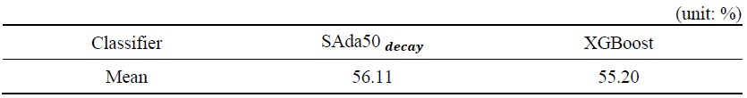
When compared with XGBoost, the stochastic AdaBoost outperformed the standard configured XGBoost model, which achieved an average of 55.20 percent weighted accuracy in the benchmark testing. XGBoost algorithm used gradient boosted trees as its voting classifier, and its performance was recorded. However, it managed to do the same task of fitting and predicting in a much shorter time. We conjecture this is because of the hardware-optimization of XGBoost, and also because it uses only decision trees as a voting component, which played a huge role in reducing the computing time of the algorithm.
IV. Conclusion
This paper pursues to find out how boosting performs in predicting very volatile financial time-series data such as stock indices, and how we can improve boosting techniques in prediction. Boosting concept is based on an ensemble scheme, where each model is added upon the previous fitting result. Since different models are combined to make a unified decision, the performance of the boosting algorithm relies heavily on the diversity of the result produced by individual base models. Two main methods of inducing diversity was proposed in this paper: one is to use heterogeneous models, and the other is to implement variable that slows convergence rate during stochastic model selection.
Stochastic AdaBoost with decaying convergence rate is proposed in this paper. Experimental results on training and testing benchmark data showed that the suggested algorithm can induce diversity as the boosting iterations intensify, and it generally performs better than the constant convergence rate algorithm. And when heterogeneous voting sets are used, the suggested algorithm substantially reduces the fitting time, while providing a similar or better performance compared with the conventional AdaBoost.
However, there is some limitation regarding this study. Although the stochastic AdaBoost with decaying convergence rate tried to reduce calculating time, it did not implement any hardware optimization. Thus, XGBoost managed to train the model in much faster time than the proposed algorithm with a reasonable degree of prediction accuracy. We believe that multi-threaded computations will lead to better time performance in stochastic AdaBoost since the individual model fitting is generally not using the entire capacity of the CPU’s computing power.
Tables & Figures
Table 1.
Raw Input Variables
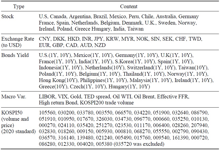
Table 2.
Permutation Importance Selected Variables
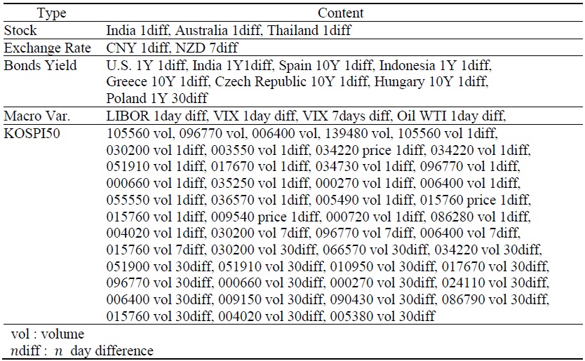
Table 3.
AdaBoost Algorithm
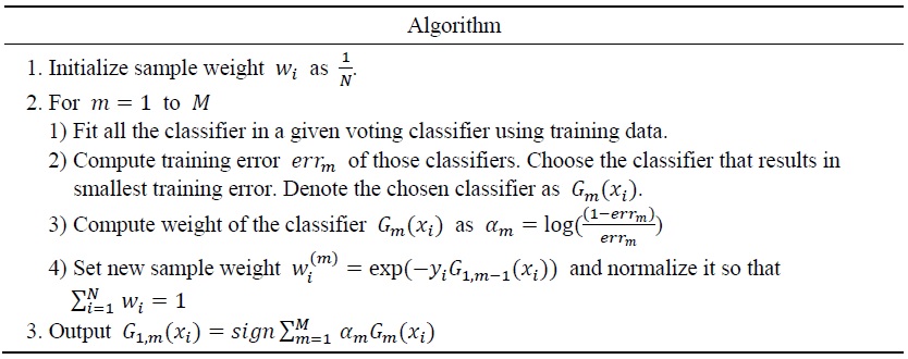
Table 4.
Gradient Boost
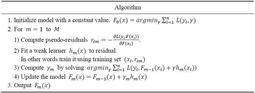
Figure 1.
Training Errors by Iteration
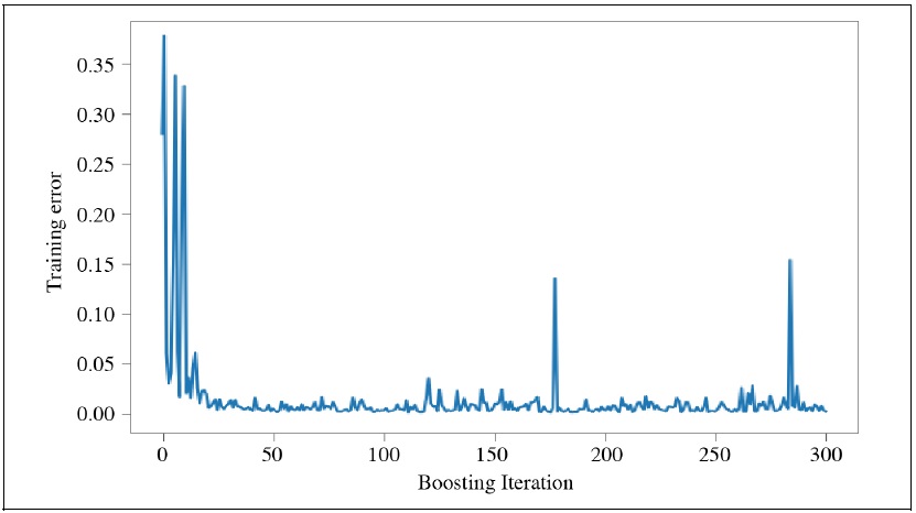
Figure 2.
Covariance between Errors (max)
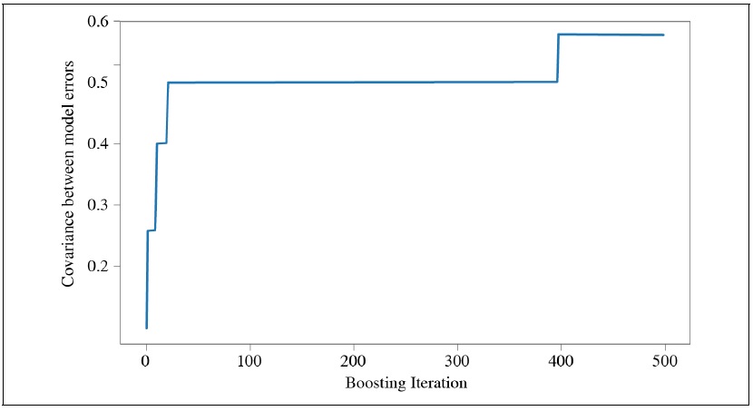
Table 5.
AdaBoost with Stochastic Algorithm Algorithm
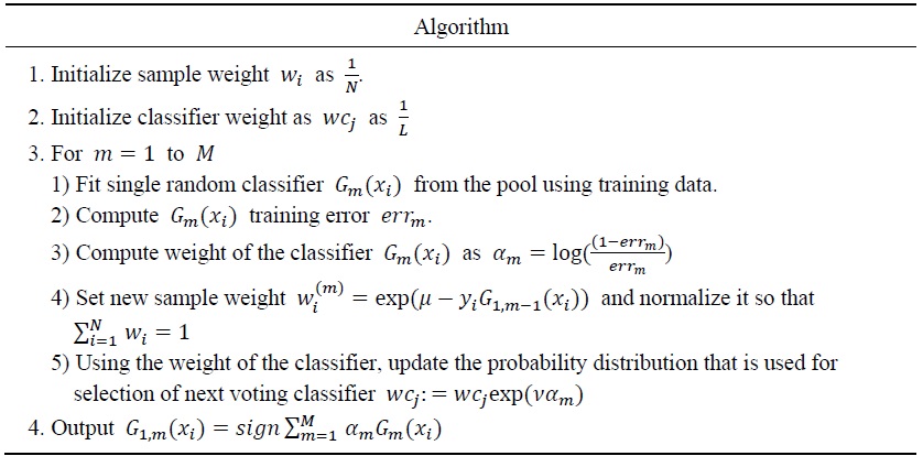
Figure 3.
Error Comparison by Configuration
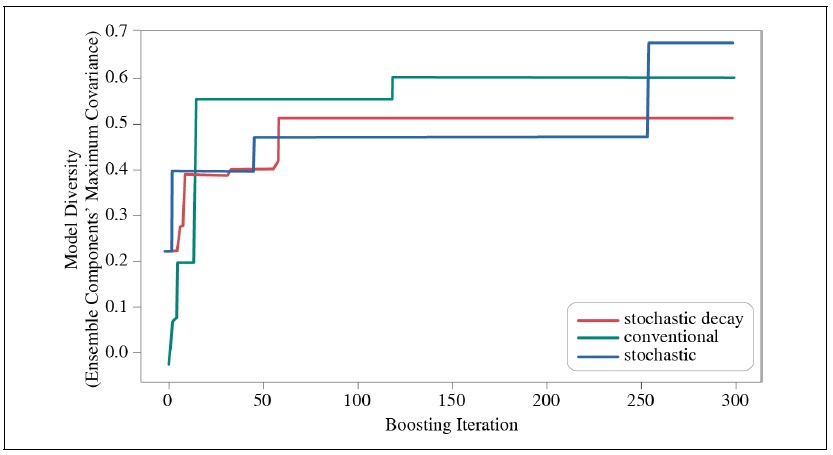
Table 6.
Classifier Accuracy by Configuration
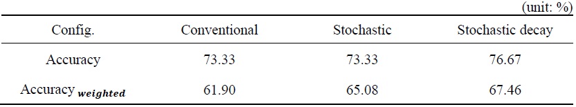
Table 7.
Benchmark Result
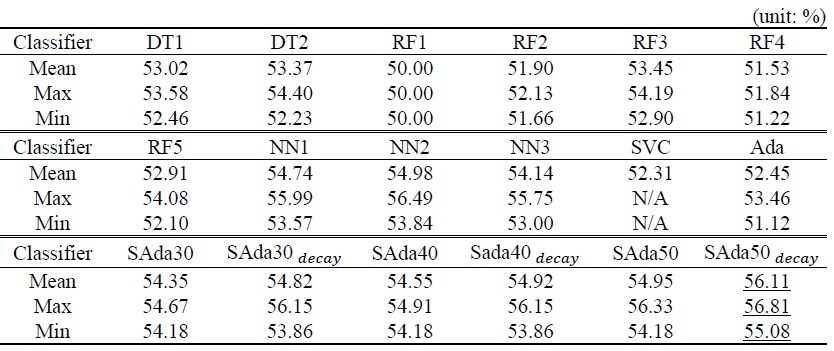
Table 8.
lassifier Accuracy
References
-
Bai, J. and S. Ng. 2009. “Boosting Diffusion Indices.”
Journal of Applied Econometrics , vol. 24, no. 4, pp. 607-629.
- Boser, B. E., Guyon, I. M. and V. N. Vapnik. 1992. “A Traning Algorithm for Optimal Margin Classifiers.” Paper presented at COLT ’92: Proceedings of 15th Annual Workshop on Computational Learning Theory, July 1992. pp. 144-152.
-
Chen, T. and C. Guestrin. 2016. “XGBoost: A Scalable Tree Boosting System.” Paper presented at KDD ’16: Proceedings of the 22nd ACM SIGKDD International Conference on Knowledge Discovery and Data Mining, San Francisco California, USA, August 13-17, 2016. arXiv:1603.02754v3.
https://doi.org/10.1145/2939672.2939785 . -
Freund, Y. and R. E. Schapire. 1997. “A Decision-theoretic Generalization of On-line Learning and an Application to Boosting.”
Journal of Computer and System Sciences , vol. 55, no. 1, pp. 119-139.
-
Guyon, I., Gunn, S., Nikravesh, M. and L. A. Zadeh. eds. 2006.
Feature Extraction: Foundations and Applications . Series Studies in Fuzziness and Soft Computing, vol. 207. Berlin: Springer. -
Hsu, K.-W. 2017. “Heterogeneous AdaBoost with Stochastic Algorithm Selection.” Paper presented at IMCOM ’17: Proceedings of the 11th Internaitonal Confernce on Ubiquitous Information Management and Communication, Jan. 2017, Beppu.
https://doi.org/10.1145/3022227.3022266 . pp. 1-8. - Huang, G., Liu, Z., Van Der Maaten, L. and K. Q. Weinberger. 2017. “Densely Connected Convolutional Networks.” In Proceedings of the 2017 IEEE Conference on Computer Vision and Pattern Recognition.
-
Li, X., Wang, L. and E. Sung. 2008. “AdaBoost with SVM-based Component Classifiers.”
Engineering Applications of Artificial Intelligence , vol. 21, no. 5, pp. 785-795.
-
McCracken, M. W. and S. Ng. 2016. “FRED-MD: A Monthly Database for Macroeconomic Research.”
Journal of Business & Economic Statistics , vol. 34, no. 4, pp. 574-589.
-
Ng, S. 2014. “Viewpoint: Boosting Recessions.”
Canadian Journal of Economics , vol. 47, no. 1, pp. 1-34.
-
Zhong, X. and D. Enke. 2019. “Predicting the Daily Return Direction of the Stock Market Using Hybrid Machine Learning Algorithms.”
Financial Innovation , vol. 5