

- EAER>
- Journal Archive>
- Contents>
- articleView
Contents
Citation
| No | Title |
|---|
Article View
East Asian Economic Review Vol. 26, No. 2, 2022. pp. 143-169.
DOI https://dx.doi.org/10.11644/KIEP.EAER.2022.26.2.408
Number of citation : 0View
71
Download
58
Revisiting a Gravity Model of Immigration: A Panel Data Analysis of Economic Determinants
|
|
Hongik University |
|---|

Abstract
This study investigates the effect of economic factors on immigration using the gravity model of immigration. Cross-sectional regression and panel data analyses are conducted from 2000 to 2019 using the OECD International Migration Database, which consists of 36 destination countries and 201 countries of origin. The Poisson pseudo-maximum-likelihood method, which can effectively correct potential biased estimates caused by zeros in the immigration data, is used for estimation. The results indicate that the economic factors strengthened after the global financial crisis. Additionally, this effect varies depending on the type of immigration (the income level of origin country). The gravity model applied to immigration performs reasonably well, but it is necessary to consider the country-specific and time-varying characteristics.
JEL Classification: F22, C51
Keywords
Gravity Model, Immigration, Poisson Pseudo-maximum Likelihood
I. Introduction
The movement of population between countries is subject to several additional constraints compared to those of capital or goods. Although the cross-border movement of capital has differed depending on the type of investment in the last few decades, when the degree of capital account openness has progressed significantly around the globe (Lane and Milesi-Ferretti, 2007), foreign investors’ capital flows through integrated financial markets are very frequent. Sometimes, capital movements are sudden, which lead to financial crises (Mendoza, 2016). Due to the extensive global value chain, the import and export of intermediate goods as well as final goods are now a common economic phenomenon (Hummels et al., 2001).
However, the scale and pattern of immigration differ among countries, as they tend to be determined by immigration policies or special relations between countries.1 In addition, with the exception of immigration determined by specific events (war refugees and international political situations);2 most immigration tends to be influenced by midto long-term trends rather than capital movements, which show high volatility in the short term.
In traditional economic theory, cross-border movement of the population has been studied, focusing on labor as a factor of production. Therefore, in this theoretical model, immigration occurs as workers move from a country with low wages to another country with high wages (Friedberg and Hunt, 1995; Card, 2001; Borjas, 2003).3 While immigration is easy to understand through this clear channel, the limitations of the theoretical model tend to be simplistic.
Immigration is not only a means of supplying labor in foreign countries, but is also closely related to the movement of one’s place of residence; therefore, immigration is affected by various factors. This study attempts to build an empirical model that explains immigration in terms of economic, geographic, historical, and cultural factors. To this end, the gravity model of trade (Tinbergen, 1962; Ball, 1967; Anderson, 1979; Deardorff, 2011) is applied to immigration; however, some explanatory variables in the traditional gravity model are replaced with explanatory variables that are relevant to immigration. After controlling for other factors, the study extends its focus on economic factors.
The OECD International Migration Database is used for this analysis. It is a bilateral country panel dataset consisting of 36 destination countries of immigration and 201 countries of origin. The analysis took place from 2000 to 2019 (annual data).4 The unbalanced panel has missing values in some country-pairs. The explanatory variables included in the gravity model are the number of population, Gross Domestic Product (GDP) per capita, distance, and dummy variables indicating neighboring countries (contiguity), common language, common colonizer, regional trade agreement (RTA), and common legal system. The gravity model of trade is a static model. Thus, the sample period is divided into two equal periods (8-year) before and after the 2008 global financial crisis (GFC). Cross-sectional regression is conducted using the average values for each period. In addition to the static model, panel data analysis to investigate the dynamics of economic factors, including time and country fixed effects is conducted.
The Poisson pseudo-maximum-likelihood (PPML) method is used to estimate the gravity model. Santos Silva and Tenreyro (2006) proposed this method. Since the standard empirical method may generate severely biased estimates resulting from zero immigrants (missing values), they propose a simple but effective method to address zeros in the immigration data.
The results of the cross-sectional regression reveal the fit (measured by R-squared) of the gravity model of trade (0.88) is higher than that of immigration. The gravity model applied to immigration reveals a model fit as high as the gravity model of trade, although it varies with the model specifications and sample periods (0.58~0.83). Population and distance are found to be closely related to immigration; this is similar to the general result in the gravity model of trade. In contrast, the control dummy variables—indicating contiguity, common language, and common colonizer—show considerable differences between the gravity models of trade and immigration.
Another cross-sectional regression was conducted for comparison with the results of a previous study, Lewer and Van den Berg (2008). In the current and previous studies, the number of population, distance, and common language are closely associated with immigration, whereas contiguity does not play an important role. The critical difference between the two studies is the result of GDP per capita, which reflects the economic factors (or motivation) of immigration. In Lewer and Van den Berg (2008), as the GDP per capita of the destination country increases relatively quickly compared with the GDP per capita of the country of origin (i.e., relative per capita GDP terms are included), immigration consistently increases. While this result is consistent with those of Lewer and Van den Berg (2008), the opposite can be seen in the current study. Thus, the current study examines the impact of the economic factors on immigration in detail through panel data analysis.
In the panel data analysis, the population and per capita GDP of destination and origin countries are separately considered instead of the multiplication of population and relative per capita GDP terms in the cross-sectional regression. Because of the panel data analysis, I find that the multiplication of population and the relative per capita GDP terms used in previous studies mask the different effects of destination and origin countries on immigration. Specifically, an increase in GDP per capita in the country of origin is associated with a decrease in immigration, whereas an increase in GDP per capita in the destination country is associated with an increase in immigration. The dominant effects vary with the type of immigration (income level of origin country and sample period). A similar result can be seen in the relationship between population and immigration.
Using panel data analysis, the study also examines whether the pattern of immigration differs before and after the GFC, and by country of origin. The analysis shows that economically motivated immigration has increased since the GFC. Economic factors are more closely associated with immigration when immigration occurs between high-income countries, whereas population changes play a relatively more important role in immigration from low- to high-income countries.
The same panel data analysis as above is also conducted by limiting the destination country to Korea in order to examine how different the effects of Korean-specific characteristics have on immigration compared with the panel data analysis results. Economic factors rather than population changes are closely associated with immigration in Korea. This trend also strengthened after the GFC. The countries of origin of immigrants to Korea are divided into low- and high-income, and the GDP per capita is estimated to be consistent with the overall panel data analysis results when the country of origin is low-income. However, when the country of origin is a high-income country, the sign is estimated to reverse or the statistical significance disappears. This can be interpreted as reflecting the Korean characteristic that most immigrants to Korea are from Asian low-income countries, leaving Korea to participate in the Korean labor market.
The study most relevant to the current study is that of Lewer and Van den Berg (2008). The authors applied the gravity model of trade to immigration. However, the sample period is different (in the current study, the data for the last 20 years are taken into consideration.). Therefore, this study uncovers new facts regarding immigration over the past 20 years. This study uses the PPML method instead of the standard empirical method, which can potentially cause biased estimators due to zero immigrants. Additionally, new empirical results are derived by classifying the effects of origin and destination countries through panel data analysis.
The remainder of this paper is organized as follows: Section II discusses our data and empirical model, Section III presents empirical results, Section IV discusses the implications of the study for South Korea and Section V concludes.
1)Great diversity in immigration across countries is mainly sourced from different immigration policies
2)A study has analyzed the economic effect of immigrants from Cuba to Miami, USA for political reasons
3)The empirical evidence is also presented in
4)In this paper, the analysis period is set after the period analyzed in the previous study,
II. Data and Empirical Model
1. Data
The number of immigrants required for empirical analysis is from the OECD International Migration Database. Immigrants are foreigners who hold a residence permit and have stayed a certain period of time (from 3 months to more than 9 months).5 The data are on inflows and outflows of foreign population, thus these are a flow variable, not a stock variable. OECD statistics not only provides information on education, occupation, and class of immigrants, but also updates that information on immigrants, by country, annually. Therefore, these data are suitable for country panel data analysis with a relatively high frequency.6 However, it should be noted that there is a limit to understanding the total number of migrants, as OECD statistics exclude those who immigrated to non-OECD countries as well as those under the age of 15 among OECD migrants (Lee, 2015).
The study comprised 36 sample countries and 201 countries of origin. Empirical analysis is carried out from 2000 to 2019;7 it is an unbalanced country panel. Table 1 presents a list of sample countries and the starting and end years of the data. Appendix Table A1 presents a list of countries of origin.
Figure 1 shows the percentage of immigrants to the total population of the 36 countries analyzed in the current study. Immigration increased rapidly after 2003 and then decreased before and after the GFC, finally falling to the level of the early 2000s in 2010. This shows that immigration tends to be procyclical and changes according to economic incentives. There was a temporary stagnant growth in immigration in 2016 following the GFC, but it rapidly increased again until 2019.
Figure 2 illustrates the proportion of immigrants to their own population (annual average percentage ratio from 2001 to 2019) in the sample countries. Among these countries, Luxembourg had the highest proportion of immigrants. This was followed by New Zealand, Iceland, Switzerland, Austria, and Germany. Mexico had the lowest immigration ratio, followed by Slovak Republic, Lithuania, Israel, and Poland. These countries have an annual average ratio of immigrants that accounts for less than 1.5% of their population. In terms of the annual average ratio, Korea is at the upper-middle level, at the 15th position among 36 countries (about 6.2%).8
Figures 3 and 4 demonstrate the change in the number of immigrants by year in Korea and the number of immigrants by country of origin, respectively. Similar to the global trend presented in Figure 1, immigrants to Korea have been steadily increasing since the 2000s; their number then decreased and stagnated before and after the GFC. Since 2012, the number of immigrants has steadily increased, reaching around 45,000 in 2019, based on OECD statistics.
The number of countries of origin for immigrants to Korea is 196, which is diverse. China accounts for an overwhelming majority with 2,586,370 immigrants alone.9 Vietnam, Korea’s top-three trading partner country, accounted for the second-largest number (481,242), followed by Thailand, the United States, the Philippines, Uzbekistan, and Indonesia as the countries sending the most immigrants to Korea. Most of the top-20 countries are from Asia, and are relatively low-income compared to Korea. An analysis of the factors affecting immigration to Korea is presented in Section IV.
2. Empirical Model
The empirical analysis consists of two main parts. In the first empirical model, the sample period is divided into two equal periods (8-year) before and after the GFC, and cross-sectional regression is performed by calculating the average values for each period. In the second empirical model, a panel data analysis is conducted to capture the average annual dynamics of immigration.
The first empirical model is Equation (1):

The subscripts
Another dummy variable indicating regional trade agreement (
We estimate the model using the PPML method, proposed by Santos Silva and Tenreyro (2006). The standard empirical method generates severely biased estimates; thus, Santos Silva and Tenreyro (2006) proposed a simple PPML method to estimate the gravity equations. This method effectively addresses the potential econometric problems resulting from heteroscedastic residuals and zero migration for some pairs of countries.
The second empirical model for the panel data analysis is presented in Equation (2):

The difference between the first and second empirical model is that the results including the product of the population of countries
5)Definitions of immigrants differ from country to country. See metadata for each sample country (
6)Another country panel data on immigration is the UN International Migration Stock. Although this database is useful for providing additional information on gender and age of immigrants, we did not use it in this study because its frequency is five-years beginning from 1990. Hence, it could not be used to analyze annual panel data.
7)In the current study, the analysis period is set after the period analyzed in the related study by
8)When interpreting
9)At least 136 countries have sent more than 100 immigrants to Korea, 79 countries have sent more than 1,000 immigrants to Korea, and 50 countries have sent more than 3,000 immigrants to Korea.
III. Empirical Result
The first empirical analysis is compared with the traditional gravity model of trade to examine how well the gravity model explains the cross-border movement of population between countries. To this end, a gravity model using trade and immigration as dependent variables is estimated. The sample period does not take into account the GFC (2008–2011). It is divided into pre- and post-crisis periods. Therefore, the precrisis period is from 2000 to 2007 and the post-crisis period from 2012 to 2019. Trade is the total amount of imports and exports during the period, and immigration is the sum of the population inflows to the destination country, denoted as country
Table 3 presents the results for the first empirical model. The fit of the gravity model of trade evaluated by Pseudo R2 is higher than that of the gravity model of immigration (0.88 vs. 0.58). This is observed both before and after the GFC. The product of the two countries' GDP per capita (the corresponding variable, the product of the population in the gravity model of immigration) and distance are statistically significant at the 1% level in both models. However, the control variables
Using another cross-sectional model, the estimation results of the current study are compared with those of Lewer and Van den Berg (2008). Three factors were considered in the comparative analysis. First, the analysis periods in the two studies differ. Lewer and Van den Berg (2008) use data from 1991 to 2000, whereas the current study uses data from after 2000 for analysis. Second, while Lewer and Van den Berg (2008) estimate a simple regression, the current study estimates the PPML method (Santos Silva and Tenreyro, 2006). Third, the sources of some explanatory variables differ, and the origin of immigration is the same as that of the OECD. The counting methods and standards may have changed by country.
Therefore, caution is needed when interpreting the results of the two studies. Nevertheless, this study contributes to the existing literature by analyzing the determinants of recent immigration by updating the dataset of the gravity model of immigration for the last 20 years.
As shown in Table 3, the analysis period is divided into before and after the GFC, excluding the GFC period (2008?2011). The explanatory variables are included in the same way as in Lewer and Van den Berg (2008). The product of the population of both countries (
Table 4 presents the estimation results of the comparison between Lewer and Van den Berg (2008) and the current study. The number of observations in both the studies is similar. As shown in Table 3,
As with the previous empirical results in Table 3,
To understand why the results on
The results of the analysis reveal that the statistical significance of the variable in the period before the GFC differs depending on the year, but statistically significant years are found to be less than zero (2001, 2002, and 2005). However, after the GFC, years with statistically significant estimation coefficients greater than zero are frequently estimated. This suggests that the economic factors affecting immigration may have strengthened after the GFC. For a more accurate estimation, a panel data analysis of the gravity model that can analyze immigration dynamics is performed.
The panel data analysis (Table 5) reveals that the sign of the estimated coefficients of
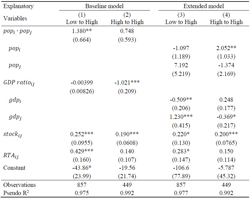
This study notes two interesting points from the analysis of the extended model in which the population and per capita GDP of countries,
In Table 6, I examine whether the explanatory variables affecting immigration are different when the country of origin is low- or high-income countries that are classified according to the 2019 World Bank classification.12 The destination countries are regarded as high-income countries based on the country classification in Table 1. The analysis shows that economic factors are highly related to immigration when the country of origin is a high-income country, which is also confirmed by the extended model. However, when the country of origin is low-income, as can be seen from the analysis results of the extended model, the increase in the population in the country of origin and the decrease in the population in the destination country are highly related to immigration than those in high-income countries.13
10)In order to control with the same number of explanatory variables as in the gravity model of trade, some control variables such as
11)
12)Upper- and lower-middle-income countries are classified as low-income countries in the current study. This is to obtain the number of observations enough for each country group for statistical inference.
13)Estimated coefficients are larger between low- and high-income countries than high- and high-income countries.
IV. Immigration to Korea
In Section IV, I conduct the same panel data analysis as in the previous section by limiting the destination country to Korea to derive implications for Korea.14 Table 7 shows the results of the baseline and extended models for immigration to Korea. This is not significantly different from the results in Table 5. Statistical significance of the estimated coefficients of
The analysis of the extended model in Table 7 when compared with the results of the extended model in Table 5 reveal that economic factors, rather than population size, are found to have a relatively higher correlation with immigration in Korea. This tendency is strengthened after the GFC. This is confirmed by the estimated coefficient of the interaction term.
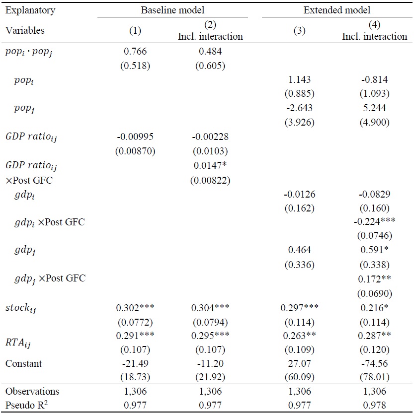
Table 8 shows the empirical results analyzing the countries of origin of immigrants in Korea by dividing them into low- and high-income countries. In the case of low-income countries, GDP per capita is estimated to be consistent with the results in Table 6. However, when the country of origin is a high-income country, the sign is estimated to be reversed or the statistical significance is found to have disappeared. This can be interpreted as reflecting the Korean characteristic: most immigrants to Korea are from low-income Asian countries (Figure 4), who leave to go to Korea to participate in the Korean labor market.
According to Hur (2017), the total number of foreigners with long-term residence status of more than one year was 158,716 as of 2016, among which the proportion of foreigners staying on a work visa (non-professional employment, visiting employment, professional manpower), overseas Koreans, and foreigners with permanent resident status was approximately 66.1%. Approximately two-thirds of all foreigners actively participate in the Korean labor market compared to Koreans. Economically motivated immigration from Asian countries is reflected in the empirical results in Tables 7 and 8.
14)The results of the cross-sectional regression limiting the destination country to only Korea are not significantly different from
V. Conclusions
This study builds an empirical model of immigration by using a gravity model. After controlling for geographic, historical, and cultural factors, it focuses on the economic factors. For the analysis, the OECD International Migration Database is used, consisting of 36 destination countries of immigration and 201 countries of origin. The analysis period is 2000–2019. Cross-sectional regression and panel data analyses are conducted. The PPML method is used to estimate the gravity model.
From the cross-sectional regression results, it is found that the gravity model applied to immigration shows a model fit as high as that of trade. Compared to previous studies, Lewer and Van den Berg (2008), it is found that economically motivated immigration had increased since the GFC.
Furthermore, a panel data analysis is conducted, wherein the population and per capita GDP of destination and origin countries are considered separately. Consequently, I find that the multiplication of population and relative per capita GDP terms used in previous studies mask the different effects of destination and origin countries on immigration. This is important, because the dominant effects vary with the income level of the country of origin. Economic factors are more closely associated with immigration when immigration occurs between high-income countries, whereas population changes play a more important role in immigration from low- to high-income countries.
The same panel data analysis as above is also conducted by limiting the destination country to Korea. Economic factors, instead of population changes, are closely associated with immigration in Korea. This trend also strengthened after the GFC. The results can be interpreted as reflecting the fact that most immigrants to Korea are from Asian low-income countries, arriving in Korea to participate in the Korean labor market.
Based on the empirical results in this study, we now come to a conclusion that the gravity model applied to immigration performs reasonably well. I leave this interesting extension and advancement of gravity model of immigration to future research.
Tables & Figures
Table 1.
Country List
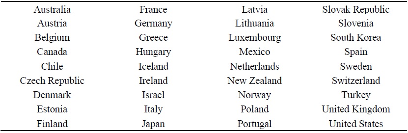
Notes: All sample countries are classified as high-income countries based on the 2019 World Bank classification, except for Mexico and Turkey. There are 201 partner countries, including those listed above. Appendix
Figure 1.
Immigrants to Population Ratio by Years from 2001 to 2019
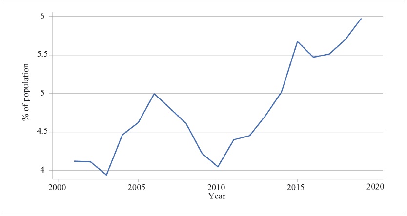
Note: The percentage ratio of total immigrants to the total population of the 36 sample countries is calculated from 2001 to 2019.
Figure 2.
Immigrants to Population Ratio by Sample Countries
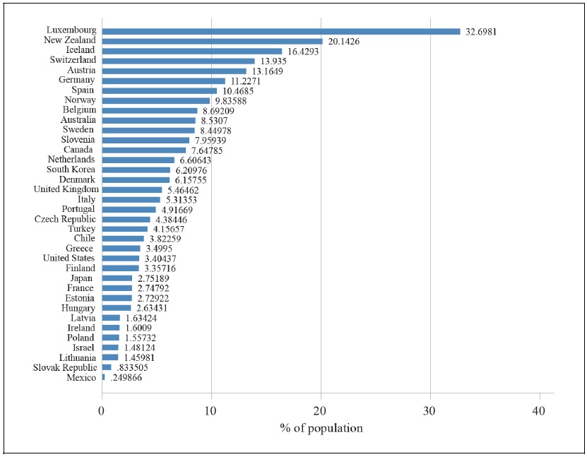
Note: The percentage ratio of immigrants to the population of the destination countries is calculated based on the annual average values from 2001 to 2019.
Figure 3.
Total Number of Immigrants to Korea by Year from 2001 to 2019
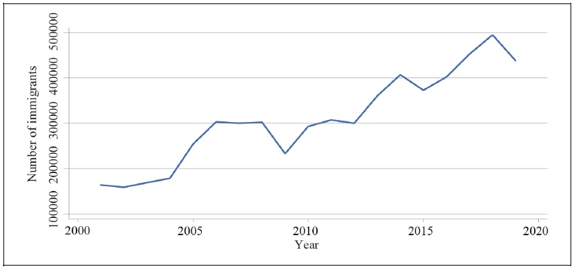
Note: The total number of immigrants to Korea is calculated by year from 2001 to 2019.
Figure 4.
Total Number of Immigrants to Korea by Country of Origin
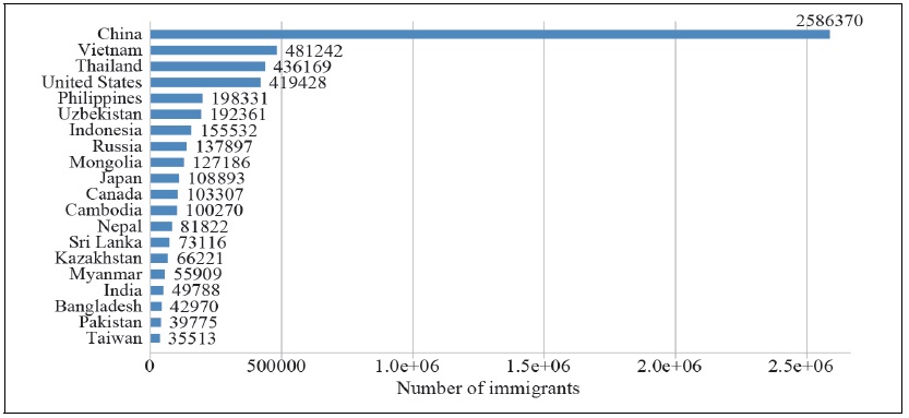
Note: The total number of immigrants to Korea is calculated from 2001 to 2019 by country of origin.
Table 2.
Basic Statistics
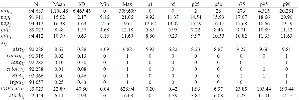
Notes:
Table 3.
Gravity Model: Trade vs. Immigration
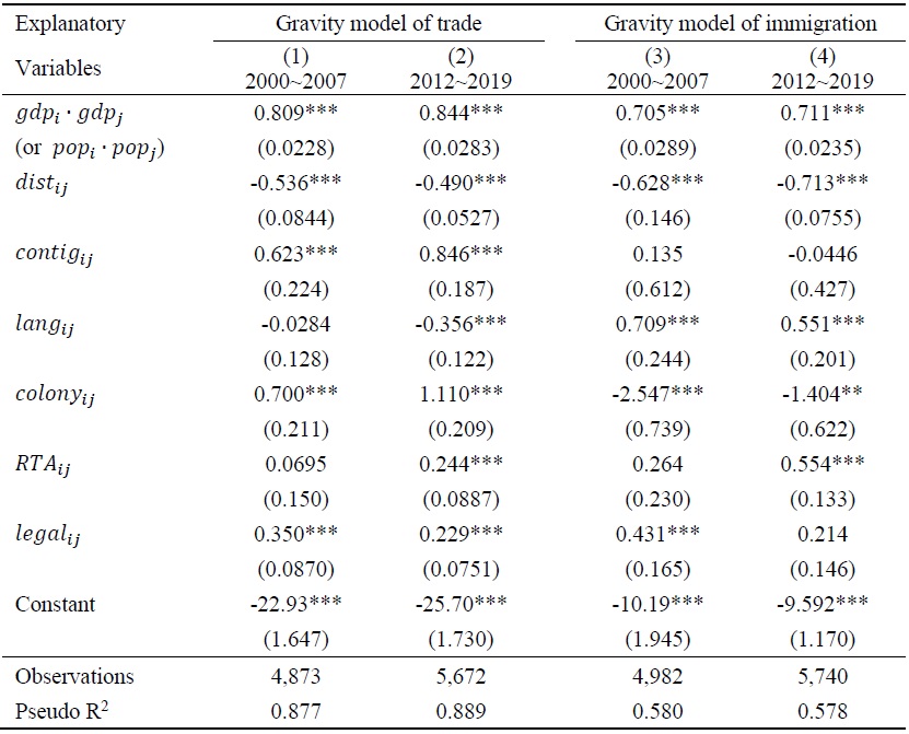
Notes: Robust standard errors are reported in parentheses. *, **, and *** indicate significance at the 10, 5, and 1-percent levels, respectively.
Table 4.
Gravity Model of Immigration from 2000 to 2019
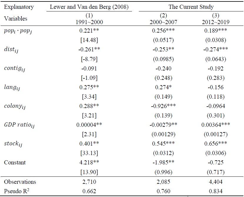
Notes: Robust standard errors are in parentheses. *, **, and *** indicate significance at the 10, 5, and 1-percent levels, respectively. 1 and 5-percent significance levels are denoted by ** in
Figure 5.
Estimated Coefficient of GDP Ratio by Years
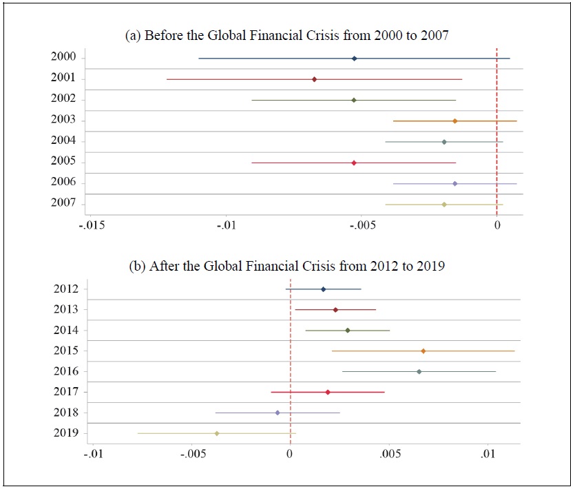
Notes: The estimated coefficient of the ratio of GDP per capita of country j to country i (
Table 5.
Panel Data Analysis: Baseline and Extended Model
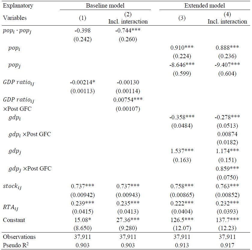
Notes: Robust standard errors are reported in parentheses. *, **, and *** indicate significance at the 10, 5, and 1-percent levels, respectively.
Table 6.
Panel Data Analysis: Immigration from Low- or High-Income Countries
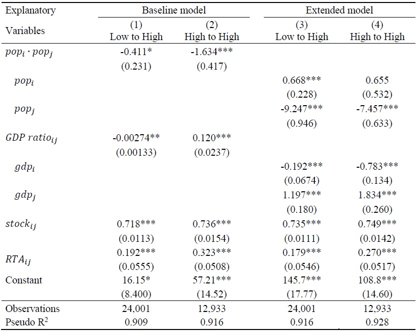
Notes: Robust standard errors are reported in parentheses. *, **, and *** indicate significance at the 10-, 5-, and 1-% levels, respectively.
Table 7.
Panel Data Analysis: Baseline and Extended Model for Korea
Notes: Robust standard errors are reported in parentheses. *, **, and *** indicate significance at the 10-, 5-, and 1-% levels, respectively.
Table 8.
Panel Data Analysis: Immigration from Low- or High-Income Countries to Korea
Notes: Robust standard errors are reported in parentheses. *, **, and *** indicate significance at the 10, 5, and 1-percent levels, respectively.
Table A1.
List of the Partner Countries
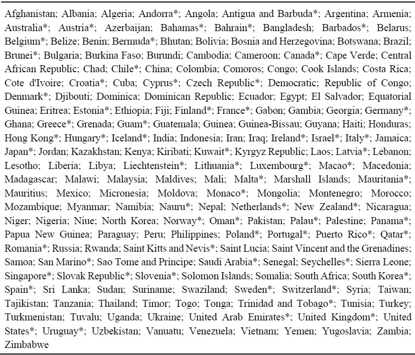
Notes: * denotes high-income countries based on the 2019 World Bank classification. The rest of the countries are low- or middle-income.
Table A2.
Gravity Model of Immigration by Years
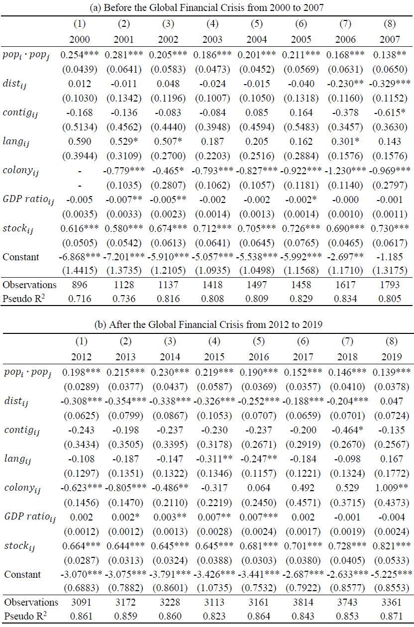
Notes: Robust standard errors are reported in parentheses. *, **, and *** indicate significance at the 10, 5, and 1-percent levels, respectively.
References
-
Anderson, J. E. 1979. “A Theoretical Foundation for the Gravity Equation.”
American Economic Review , vol. 69, no. 1, pp. 106-116. -
Ball, R. J. 1967. “An Econometric Study of International Trade Flows.”
Economic Journal , vol. 77, no. 306, pp. 366-368.http://doi.org/10.2307/2229319 
- Borjas, G. J. 1999. “Economic Research on the Determinants of Immigration: Lessons for the European Union.” World Bank Technical Paper, no. 438.
-
Borjas, G. J. 2003. “The labor demand curve is downward sloping: Reexamining the impact of immigration on the labor market.”
Quarterly Journal of Economics , vol. 118, no. 4, pp. 1335-1374.
-
Card, D. 1990. “The impact of the Mariel boatlift on the Miami labor market.”
Industrial Labor Relations Review , vol. 43, no. 2. pp. 245-257.
-
Card, D. 2001. “Immigrant inflows, native outflows, and the local labor market impacts of higher immigration.”
Journal of Labor Economics , vol. 19, no. 1, pp. 22-64.
-
Deardorff, A. V. 2011. “Determinants of bilateral trade: does gravity work in a neoclassical world?” In Stern, R. M. (eds.)
Comparative Advantage, Growth, and the Gains from Trade and Globalization-A Festschrift in Honor of Alan V Deardorff . Singapore: World Scientific Publishing Co. Pte. Ltd. pp. 267-293. -
de Haas, H., Czaika, M., Flahaux, M.-L., Mahendra, E., Natter, K., Vezzoli, S. and M. Villares-Varela. 2019. “International Migration: Trends, Determinants, and Policy Effects.”
Population and Development Review , vol. 45, no. 4, pp. 885-922.http://doi.org/10.1111/padr.12291
-
Friedberg, R. M. and J. Hunt. 1995. “The impact of immigrants on host country wages, employment and growth.”
Journal of Economic Perspectives , vol. 9, no. 2, pp. 23-44.http://doi.org/10.4324/9781315054193-4
-
Gandal, N., Hanson, G. H. and M. J. Slaughter. 2004. “Technology, trade, and adjustment to immigration in Israel.”
European Economic Review , vol. 48, no. 2, pp. 403-428.http://doi.org/10.1016/S0014-2921(02)00265-9
-
Hummels, D., Ishii, J. and K.-M. Yi. 2001. “The Nature and Growth of Vertical Specialization in World Trade.”
Journal of International Economics , vol. 54, no. 1, pp. 75-96.
- Hur, J. 2017. “Fiscal Implications of Immigration Policy in Korea.” KDI Policy Study, no. 2017-20. Korea Development Institute.
-
Lane, P. R. and G. M. Milesi-Ferretti. 2007. “The external wealth of nations mark II: Revised and extended estimates of foreign assets and liabilities, 1970-2004.”
Journal of International Economics , vol. 73, no. 2, pp. 223-250.http://doi.org/10.1016/j.jinteco.2007.02.003
- Lee, C. W. 2015 “Statistics on Korean Emigration: Current State and Limitations.” IOM MRTC Policy Report Series, no. 2015-04, Migration Research & Training Centre. (in Korean)
-
Lewer, J. J. and H. Van den Berg. 2008. “A gravity model of immigration.”
Economics Letters , vol. 99, no. 1, pp. 164-167.http://doi.org/10.1016/j.econlet.2007.06.019
-
Mendoza, E. G. 2016. “Sudden Stops, Financial Crises, and Leverage.”
American Economic Review , vol. 100, no. 5, pp. 1941-1966.
-
Santos Silva, J. M. C. and S. Tenreyro. 2006. “The Log of Gravity.”
Review of Economics and Statistics , vol. 88, no. 4, pp. 641-658.http://doi.org/10.1162/rest.88.4.641
-
Taylor, A. M. and J. G. Williamson. 1997. “Convergence in the age of mass migration.”
European Review of Economic History , vol. 1, no. 1, pp. 27-63.http://doi.org/10.1017/s1361491697000038
-
Tinbergen, J. 1962.
Shaping the World Econom: Suggestions for an international Economic Policy . New York: The Twentieth Century Fund.