

- EAER>
- Journal Archive>
- Contents>
- articleView
Contents
Citation
| No | Title |
|---|---|
| 1 | Digital financial inclusion and income inequality nexus: Can technology innovation and infrastructure development help in achieving sustainable development goals? / 2024 / Technology in Society / vol.76, pp.102411 / |
Article View
East Asian Economic Review Vol. 26, No. 4, 2022. pp. 305-336.
DOI https://dx.doi.org/10.11644/KIEP.EAER.2022.26.4.415
Number of citation : 1View
58
Download
51
Infrastructure Integration, Poverty, and Inequality in Developing Countries: A Case Study of BRI Transport in the Lao PDR
|
|
Waseda University |
|---|

Abstract
This study applied the macro–micro simulation model (i.e., what-if analysis) to investigate the impact of transport related to the Belt and Road Initiative (BRI) on poverty and income inequality in Laos. We selected Laos as a case study of a developing country. We used the standard GTAP model with the GTAP database (version 10) for the macrosimulation, whereas we used the household model with the latest Lao household data from 2019 for the microsimulation. Our findings revealed that the output of the Lao economy was anticipated to increase by up to 0.3%, while the poverty rate was anticipated to decline from 17.0% to 15.7%. However, there would be winners and losers in industries and groups of households in different areas. In particular, rich households with a comparative socioeconomic advantage, such as in education, engagement in nonfarm business, and infrastructure access, would mostly gain benefits; consequently, this would lead to higher inequality in Laos. Therefore, the inequality index (i.e., the Gini coefficient) would increase from 41.2 to 60.1. After a simulation of BRI transport, we also found that some nonpoor households, which are mainly associated with farm activities and lower educational levels, would fall into poverty.
JEL Classification: D58, D63, F14, F15
Keywords
Laos, Macro–micro model, Belt and Road Initiative (BRI), Inequality, Poverty
I. Introduction
In March 2022, the Lao People’s Democratic Republic (PDR), or Laos, become one of 147 countries that endorse China’s Belt and Road Initiative (BRI) since its introduction in 2013 (Nedopil, 2022). The cooperation on the BRI between Laos and China, as with several other BRI countries, has been highly evident since the end of 2016. This is when the Lao PDR government signed a memorandum of understanding (MoU) and several cooperation documents with China in various areas with the aim of supporting the BRI. The most crucial documents include the master plan of cooperation and the Laos-China Economic Corridor (LCEC) Cooperation Framework, which provide a guiding direction for the BRI’s development between Laos and China in several areas. These areas include infrastructure, agriculture, capacity building, industrial parks, culture and tourism, finance and banking, and production promotion (Lao and Chinese Government, 2017, 2019). In addition, some infrastructure mega construction projects for connecting China and Laos are underway. In particular, the Laos-China railway project, with a total investment value of US$5.9 billion, is the top priority for the BRI cooperation between the two countries. Recently, the railway construction of both the Chinese and Lao sections was completed, and the transport service officially opened in early December 2021. It is part of a regional railway network called the Singapore-Kunming High-Speed Rail Link along the China?Indochina Peninsula Corridor.1 The Laos-China railway is expected to bring benefits not only to Laos and China but also to other countries in the region, including Cambodia, Malaysia, and Thailand.
For Laos, as a small, land-locked, open economy rich in natural resources, engaging in the BRI is a strategy for overcoming the disadvantages of its geographic location through transforming from a “land-locked” to a “land-linked” country. Between 2000 and 2020, Laos recorded high economic growth of 7.4% on average (Lao Statistics Bureau, 2012); however, this growth was largely driven by the boom of resource industries, such as mining and hydropower, where employment opportunities are limited. Thus, most of the country’s population of approximately 7 million people, who are largely employed or engaged in the agricultural sector, might not benefit from the resource sector. Consequently, the contribution of such high economic growth to poverty reduction is limited resulting in low growth elasticity of poverty (0.71) which is lower than its regional peers such as Vietnam (1.33) and Indonesia (1.76) (Lao Statistics Bureau and World Bank, 2020, p. 22).
Furthermore, Laos is one of the poorest countries in the region, and many farm households remain in poverty. In 2018, the national poverty rate was 18.3%, which is higher than that of neighbors such as Cambodia (13.5%), and Vietnam (6.8%); only the poverty rate of Myanmar is higher (24.8%; ASEAN Secretariat, 2020, p. 28). In this regard, the Lao government considers poverty reduction to be among its top priorities for long-term development; thus, it considers the transport connectivity provided through the BRI to be beneficial for promoting trade, production, and job creation for local people (Lao and Chinese Government, 2019, p. 4). The expansion of transport connectivity is expected to encourage economic growth and poverty reduction in Laos, since empirical evidence has suggested that road transport development, for instance, significantly contributes to economic growth and poverty reduction (Ghani et al., 2016; Warr, 2005). Such development also has a significant effect on poverty reduction in rural areas through improving the well-being of people, increasing their income through nonagricultural production, and generating employment opportunities (Asian Institute of Transport Development, 2011; Gachassin et al., 2010; Gibson and Rozelle, 2003; Lord, 2010).
However, the implications of the BRI transport connectivity initiative may include trade-offs between costs and gains within and across various economic sectors and social groups, especially the poor in different regions of Laos. Therefore, careful analysis of the potential economic impacts is required, including transmission channels. Based on the findings, various policy options should be identified to ensure that the development of BRI transport infrastructure can help Laos to accelerate the reduction of poverty and inequality; moreover, such development should help it to advance toward Sustainable Development Goals (SDGs) 1 (no poverty) and 10 (reduced inequality) by 2030. Furthermore, relevant studies have not yet quantitatively assessed BRI transport’s effect on poverty reduction and inequality at the household level, at least in Laos. Therefore, the present study aimed to contribute to the understanding of the connection between BRI transport infrastructure, poverty, and inequality at the household level in the context of Laos. This study also differs from previous literature as it applied the top-down macro–micro simulation model with the latest household data from 2019. This was expected to yield richer results, discussions, and implications for the literature on Laos as a case study of a developing country.
In terms of policy implications, based on the findings, reducing poverty as well as inequality across regions requires not only local infrastructure and institutions to be improved, besides the BRI transport, but also education, training, market information (including the labor market), and entrepreneurship capacity. This will allow local households and businesses to adapt or adjust their behaviors to the new environment to improve their productivity and competence. Special attention should be paid to low-income households and regions with high poverty rates. If benefits or income could be redistributed toward lower-income groups, poverty reduction would be much higher and inequality (or the Gini index) would be reduced simultaneously. To this end, the revenue derived from BRI transport and beneficial industrial sectors (i.e., the extraction and service sectors) should be redistributed to finance and facilitate the development of low-income households in poor regions. Furthermore, increasing the progressive income tax rate, especially for the richest households, could be an alternative policy for income redistribution, potentially reducing income inequality directly.
The remainder of this paper is organized as follows: Section II reviews the literature related to the links between the BRI, economic growth, and poverty reduction among others. Section III presents the methodology employed to conduct this study, including analytical approaches based on the Global Trade Analysis Project (GTAP) model and the household model. Section IV describes the data source, while Section V presents the key findings and discussion. Lastly, Section VI summarizes the results and provides policy implications.
1)The China-Indochina Peninsula Corridor is one of six BRI economic corridors under the Silk Road Economic Belt of BRI are (1) the New Eurasian Land Bridge; (2) the China-Central Asia-West Asia Corridor; (3) the China-Pakistan Corridor; (4) the Bangladesh-China- Myanmar Corridor; (5) the China-Mongolia-Russia Corridor; and (6) the China-Indochina Peninsula Corridor.
II. Literature Review
Since its announcement by the Chinese president in 2013, the BRI has gained the attention of numerous stakeholders, including those in academia. Accordingly, much research has been conducted on the BRI across more than 100 disciplines. These studies have mainly aimed to assess the impact of the BRI on business and economics in BRI countries (including Laos) as well as non-BRI countries at the macro level (Cao and Alon, 2020). However, only a few studies have evaluated the BRI’s impact at the local economic or household level. The methodologies commonly used by previous research are dominated by simulation analysis (what-if) rather than empirical analysis (after the fact), since many areas of the BRI are still being negotiated, planned, and processed, or they have not been fully implemented.
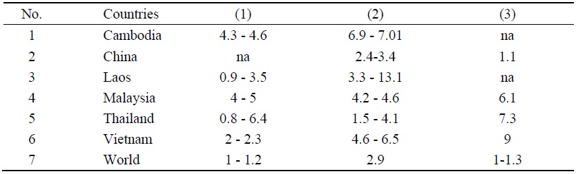
Notably, previous simulation research has largely applied the computable general equilibrium (CGE) model using the GTAP database to investigate the impacts of the BRI, such as transport infrastructure development, on economy and trade. The basic key assumptions of the CGE model are that all agents are price takers in a perfect market, where firms maximize their profit while consumers maximize their utility of consumption, and labor mobility exists perfectly across industries. Some research findings regarding the BRI’s impact on economies are selectively reported in Table 1.
In general, the results regarding the BRI’s impact on the world economy differ, ranging from 1% to 2.9%. Such a nuanced gap in results is due to the identified specification of the model, since some studies have extended the specification of the standard model by including more dimensions and different assumptions for their scenario analysis. In particular, the research on the BRI’s effect on Laos has found that the impact of BRI infrastructure would accelerate the country’s economy by 0.9-3.5% from the baseline scenario (Maliszewska and van der Mensbrugghe, 2019). However, compared with neighboring countries, such as Cambodia and Thailand, the net benefit seems to be lower compared with a large value investment from the BRI in respect of the size of the Lao economy. According to Bandiera and Tsiropoulos (2020), the total investment of the BRI in Laos is equal to 140% of its GDP, whereas it was less than 60% and 5% in Cambodia and Thailand, respectively. According to de Soyres et al. (2020), Laos could gain further, besides trade cost reductions, if trade facilitation is considerably improved.
In one of the most recent studies, de Soyres et al. (2020) apply the structural computable general equilibrium model to investigate the effects of transport cost reduction on trade, welfare, and gross domestic product (GDP) in the context of the government budget financing the BRI investment (i.e., the cost of the project) through raising taxes. In total, they use observations from 107 countries, including 55 BRI countries. Their findings indicate that investment in BRI infrastructure would grow the economy by up to 3.4% in BRI countries, while non-BRI economies would also benefit by up to 2.6% through the channel of economic integration. Overall, the global economy would grow by 2.9%. However, some countries, including Azerbaijan, Mongolia, and Tajikistan, may suffer negative net welfare due to the high cost of investment over gains. Finally, as asserted by this study, further benefits could be achieved if countries participating in the BRI could reduce delays at their borders, reduce tariffs by half, or through a combination of policy reforms.
Maliszewska and van der Mensbrugghe (2019) provide more notable findings on the BRI, not only in the economic dimension but also regarding poverty and the environment. While their study is grounded on the CGE model, it differs from the aforementioned study in the model in a way that it specifies fewer structural economic sectors without projects financed by tax or budget. Therefore, the effect of the BRI is found to be lower at 0.7%. Although their study provides poverty reduction figures as well as an increase in global CO2 emissions due to the BRI, it fails to provide clear details on the channel effect on poverty reduction. For Laos, the study indicates that the country is expected to be one of the largest beneficiaries of the BRI, along with Kyrgyzstan, Kazakhstan, Ethiopia, and Cambodia, due to a large reduction in transport costs. Specific industries, such as extractive sectors, leather goods, chemicals, rubber and plastics, and fabricated metal products, should witness a significant boom, while transport and other service sectors would see moderate growth. On the other hand, agriculture, clothing, apparel, and processed food exports would be the hardest hit or losers.
Although the abovementioned studies have provided some insights, detailed analyses at the local economic or household level are still missing. Bird et al. (2020) and Lall and Lebrand (2020) have extended the analysis of the CGE model at the district level in China and countries in Central Asia, such as Kazakhstan, Uzbekistan, and Kyrgyzstan. Their studies are considered a useful reference for the present study as we apply our analysis at the micro level. Lall and Lebrand (2020) find that BRI transport investments would facilitate economic development in larger urban districts located near trade hubs along transport corridors; by contrast, they find that people living in districts that are more distant from such hubs would tend to lose out because of the outflow of labor and the loss of competitiveness of industries. Therefore, people residing in trade hubs or near transport corridors would tend to gain relatively more from the economic opportunities. The authors suggest that improving the domestic transport networks within countries would help to spread the benefits to people in areas far from the transport corridors through ensuring better access to cheap imports and labor mobility. The major advantage of their study is the inclusion of a flexible assumption in the model, allowing monopolistic competition and labor mobility across regions, which should reflect the realities more accurately than previous studies.
III. Methodology
This study applies a quantitative analysis that follows the macro-micro simulation model to understand and quantify the impact of BRI transport on poverty and income distribution at the household level. There are two steps to conducting macro?micro simulation: The first step involves using a macro model to produce macrosimulation results, while the second step involves applying a micro or household model to perform a microsimulation analysis based on the exogenous inputs taken from the macrosimulation results. In the first step, we apply the existing macro model of the GTAP for our macrosimulation analysis. The GTAP model is a multi-region model developed by Corong et al. (2017), which has been well documented in the academic literature.2 It is generally used to study the issues in a context or that involve trade liberalization or trade policies. Nevertheless, the model has received some criticisms due to its complexities or black box, as several equations and variables move simultaneously (Burfisher, 2021, p. 287).
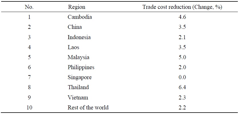
Kyophilavong et al. (2016) use the standard static GTAP model with version 8 of the GTAP database to analyze the impact of trade policies on the Lao economy. Our research varies from such previous studies in the context of Laos by employing the latest GTAP database, which is version 10 at the time of our study. To estimate the impact of BRI transport on Laos and other ASEAN economies, we assume that BRI transport development, such as sea, rail, and road, would reduce trade costs as a shock scenario (what-if), which would then influence the flow of trade, the economy, and welfare. Here, we refer to the value of international trade cost reduction3 in BRI and non-BRI countries estimated by de Soyres et al. (2020), as reported in Table 2. We do so because their estimation is regarded as the most comprehensive and available for international comparison at the time of our study. Specifically, Thailand, Malaysia, Cambodia, China, and Laos are the beneficiaries of the largest trade cost reductions from enhanced transport connectivity through the BRI.
In the second step of our analysis, we apply a micro model to investigate the impact of BRI transport on poverty and income distribution (Gini coefficient index) at the regional and household levels in Laos. To this end, we use the changes in four variables of GDP or output, employment, price, and wage as exogenous inputs to connect our macro- and micro-simulation models. In this regard, one could argue that the microsimulation results are critically dependent on or limited by the specifications, assumptions, and results of the GTAP model. Here, the methodology of the microsimulation model in the second step mainly follows the top-down behavior (TBD) approach4 of Tiberti et al. (2018). Accordingly, equations (1), (2), (3), and (4) below briefly demonstrate the major economic behaviors of households for their occupation, business activities, and consumption in the microsimulation model.5 Equation (1) is as follows:
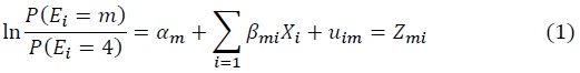
where
First, equation (1) demonstrates that the probability of being employed in different occupations is conditional on individual characteristics, especially education or skills, experience or age, gender, and location. Here, there are four occupation categories, namely wage sector, self-employed in nonfarming, self-employed in farming or farmers, and unemployed/not working. Equation (1) and its parameters are estimated using a multinomial logistic regression. The results of the regression are reported in the Appendix. For the simulation analysis, the job queuing approach follows, which allows household members to shift or move across occupations based on their probability values. For instance, the position of an individual’s occupation could change from unemployed to employed in the wage sector subject to his/her highest value of probability of being employed when job vacancies exist in the wage sector due to the impact of BRI transport development. As a result, household members (individuals) could receive more wages from employment as a part of their income and vice versa. In this regard, the estimation of occupational probability is crucial for poverty analysis at the household level. Equation (2) is as follows:

where  is business profit in the local currency for household
  is the number of skilled laborers in sector
  is the number of unskilled laborers in sector
Since some households operate businesses, including farms and nonfarm businesses, profits could be a part of their income. To capture this source of income, equation (2) identifies the profit function for a household’s business, which is estimated through OLS regression. The regression results are displayed in the Appendix. They demonstrate that the profit is mainly influenced by the number of skilled and unskilled laborers and the education of the household head, since the operation of the business is predominantly managed by the household head. To simulate the profit income, a change of employment (increase or decrease in the numbers of skilled and unskilled laborers) generated in the labor market in equation (1) would consequently feed into the profit function. For instance, if the number of laborers, both skilled and unskilled, increases because of BRI transport for household
After the estimation of equations (1) and (2), household total income can be simulated using equation (3). Equation (3) is as follows:

where  is the wage income of labor
  is profit income for household
  is other sources of income for household
Equation (3) clearly demonstrates that a household’s income comprises wages derived from employment in the wage sector, business profit, and other sources, such as social welfare, remittances, dividends, and rents. For the other sources of income, we assume them to be constant. Equation (4) is as follows:
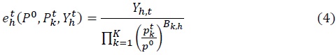
where  is the equivalent income function specific to household
  is the price of commodity
Finally, as demonstrated by equation (4), the real expenditure is produced based on the income derived from the previous equations and the price index at the commodity prices weighted by the budget share. Crucially, it illustrates whether a household will be better or worse off; it is not dependent on income only but also a proportion of the budget spent on commodities and their prices in the market. Therefore, an increase in real expenditure due to income or lower prices could help a household to escape from poverty and vice versa. Lastly, one of the main properties of the microsimulation is the value of the individual residual term for equation (1). Accordingly, we run the estimation for more than 90,000 iterations for each of 20 simulations in total and then take the mean value as the result.
2)Since the standard GTAP model comprises of several blocks of behavioral equations and assumptions for different agents, the details of these specifications are excluded in this paper to save the space but can be reviewed on
3)The trade cost consists of tariff, transport, and time cost. There are two values for trade cost reduction subjected to the assumption for the lower and upper bounds. Our study uses the cost reduction result from the upper bound assumption for GTAP simulation since the upper bound assumption is more realistic than the lower bound. Note that the assumption used for the lower bound is based on the fixed transport mode such as railway, in which the transport cost will be reduced only when there is an investment on the new railway or an upgrade of the existing railway. On the other hand, the assumption used for the upper bound is more flexible based on the ability to switch between transport modes, meaning that a country can choose between different transport modes such as from sea transport to rail transport, if the transport cost of the rail is lower.
4)We also utilized the STATA code and toolkit for the exercise of our analysis which are accessible and downloadable. More details, see on following link:
5)More details, please see on
6)The definition of skilled labor is reflected based on the data from LECS 6 as it indicates that more than 60% of total labors in nonfarm business has education level of junior high school. Therefore, the education level of junior high school is considered as the threshold for defining the skilled labor. Similarly, almost 70% of total farm labor had education level at primary school. Therefore, primary school is the benchmark for defining skilled labor in farm business.
IV. Data Sources
To link the GTAP model and the micro model, we perform data matching between the GTAP database and the household data from the Lao Expenditure and Consumption Survey (LECS). The GTAP database is a global database that is initiated, maintained, and updated by the Center for Global Trade Analysis at Purdue University. It demonstrates the patterns of trade, production, consumption, and service among regional and individual economies. Currently, there are 10 versions of the database, the latest of which at the time of our study is version 10. The LECS is a nationally representative survey of randomly selected households that enables the Lao government to estimate the poverty rate at the national and local levels. The LECS is conducted every 5 years by the Lao Statistics Bureau (LSB) and is funded by the Lao government and international donors. Six rounds of the survey have been conducted since 1992, with samples ranging from 2,868 households (LECS 1) to 10,176 households in 2019 (LECS 6).
In our study, we use the latest data from version 10 of the GTAP database and the LECS 6. Due to the complexity of the microsimulation model and the limitations of household data, we match these two databases with four economic activities,7 namely (1) wage sector, (2) self-employed in nonfarm, (3) self-employed in farming or agriculture, and (4) unemployment, including not working. Hence, we aggregate the simulation results of the GTAP model from 10 sectors initially in the first step into three sectors, namely the wage sector, self-employed in the farm sector, and selfemployed in the nonfarm sector. Then, we adjust them by the pattern of household employment by skills and industries in the second step. Similarly, as 29 items of commodities consumed by households are recorded in the LECS 6, we expand the simulation results of the GTAP model from 10 commodities initially in the first step to 29 commodities for matching, which are reported in the Appendix. We also match employment and wage by laborers’ skills and economic activities between the two simulation models.
Since we use household data from the LECS 6 for our poverty and income distribution analysis, we briefly summarize the statistics in Table 3 to demonstrate the structure of households’ characteristics and their economies.
Note that the results of the average summary statistics for households in the LECS are comparable to the national average summary statistics at the national level, since the design of the representative household survey of the LECS is based on the population census survey.8 Accordingly, approximately a quarter of the sampled households reside in urban areas, whereas the majority live in rural areas. The average household size is approximately five individuals living under the same roof, sharing social and economic benefits, which is slightly higher than in neighboring countries, such as Thailand (3.7 individuals), Vietnam (3.8 individuals), and Cambodia (4.6 individuals; United Nations, 2017, pp. 18-19).
The largest household sizes are in rural areas, especially in the Northern region. Within the households, two to three people or half of the household members work as employees, self-employed, or farmers in private businesses and public services for earning wages or salaries, which is one of their main forms of income. Moreover, the business profit is comparable as a source of income for a group of households that run nonfarm businesses, which account for 12% of the sampled households. Nonfarm businesses, as occupied by small enterprises, involve wholesale, retail, restaurants, hotels, and processing manufacturing. For farm businesses, the monthly average profit is relatively low due to low productivity or the cost of production; for example, the prices of fertilizer, oil, and animal feed are relatively high and have exhibited an upward trend in recent years resulting in lower profit. Accordingly, farm households are relatively poorer and many are in poverty, which is mainly attributed to the national poverty rate as 72% of people are engaged in agriculture. Most farmers mainly produce paddy rice (two harvests a year), maize, cassava, coffee, tea, rubber, fish, poultry (chicken, ducks, and turkeys), and livestock (cattle, buffalos, pigs, and goats). In 2019, the agricultural sector accounted for 15.20% of the GDP and mainly exported to China, Vietnam, and Thailand (Lao Statistics Bureau, 2019, p. 84; Insisienmay et al., 2019, p. 8).
Remittances, as the third major form of income, account for over 14.4% of total income. Regarding education, most household members, including the household head, have a low educational level of primary or junior high school. In this regard, most household members are considered unskilled laborers mainly employed in the agricultural, construction, and manufacturing sectors, while the minority of skilled household members work in public sectors, such as government agencies. In terms of the absolute poverty rate, 17% of total households live under the poverty line,9 which means that they consume goods and services below the poverty line of 280,910 Kip or US$3010 per month, equivalent to the minimum required consumption of 2,100 Kcal per day, basic education, and health that are necessary for living. This poverty measurement is based on food and nonfood consumption (Lao Statistics Bureau and World Bank, 2020, pp. 59-63). The data also indicate that households spend more than half of their budget on food, such as rice, vegetables, and meat. Another expense is transport and communication, which combined account for more than 11% of total consumption, while less than 5% is spent on other nonfood items. In this respect, the price changes of such food commodities as well as transport would greatly affect real income, real expenditure, as well as households’ position in poverty.
7)This is because the numbers of observations or samples, especially skilled and unskilled laborers in some industries such as extraction, utilities, media and entertainment, transport and communication, hotel and restaurant, and construction are small and insufficient for the econometric estimation and micro-simulation. Therefore, we aggregate the economic activities into 4 sectors to satisfy the micro-simulation estimation.
8)Population census survey is conducted in every 10 years and the latest survey was the population census survey 2015.
9)Note that this poverty rate is lower than the announcement of the official poverty rate (18.3%), because of the data access limitation under the statistics law. There were 10,028 households in total, but 60% of the database, or 6,017 households or 29,236 individuals can only be accessed.
10)Based on the exchange rate from BCEL on 16th March 2021, which is 9,362 kip/USD for buying rate.
V. Results and Discussion
1. Impact of the BRI Transport on the Lao Economy
Laos is among the top three economies that stand to gain the most from the BRI, besides Cambodia and Thailand, due to a relatively large trade cost reduction and the strong growth in resource and service industries (Figure 1). The reduction of trade costs will encourage exports to and investment in ASEAN countries and China, especially industries with a comparative advantage, such as the extraction and tourism industries in Laos and the construction and agricultural industries in Thailand. By contrast, Singapore is the only ASEAN country that is projected to lose in terms of welfare and economic gains. The decline of Singapore’s GDP and welfare is largely due to the loss of comparative advantage in transportation. This is because there would be no further trade cost reductions for Singapore, since its transport system is already well established, whereas other countries will benefit from trade cost reductions due to improved transport. Consequently, Singapore will see a decline in some services and construction. Similarly, the rest of the world will experience a slight fall in GDP due to the outflow of capital investment into the ASEAN region; however, it will still witness a somewhat of a gain in welfare because of efficient resource allocation and technical change, which will increase consumption.
Although the Lao economy is expected to see an increase in GDP of 0.32%, the benefits would not be equally distributed among industries. There will be winners and losers. As reported in Table 4, the extraction industry is expected to grow significantly by more than 8%, which is much higher than other industries. As Laos is rich in natural resources, including those extracted by mining, the extraction industry has become one of the most competitive sectors in Laos. The high growth of the extraction industry is driven by a strong demand for the resources in China and Vietnam. This reflects the resource allocation of raw materials or inputs from developing countries (e.g., Laos) to feed the manufacturing industries in emerging economies, especially China, since most exports from Laos in this sector are primary products, such as mineral ore. The exports of the extraction industry are expected to gain approximately US$50 million.
Moreover, service industries related to tourism, including hotels, restaurants, wholesale, and entertainment, are growing at a far less positive rate. By contrast, the agriculture, manufacturing, and utility industries will experience a decline in production from -0.08% to -0.2% because of the influx of imported goods due to cheaper prices and labor mobility – especially the outflow of skilled workers to high-growth industries (e.g., extraction and service). In the agricultural sector, the exports will increase by almost 1%, but the imports could be raised higher by 3.56%, leading to a decline in the overall agricultural output. Hence, the expected contraction of the three industries, including agriculture, due to BRI transport would affect many households, or approximately 70% and 4% of total laborers currently working in the agriculture and manufacturing industries, respectively.
In reality, a concern exists regarding the transition of labor mobility, especially the movement of labor from the agricultural sector to other industries, which might not occur as smoothly as the perfect labor mobility assumed by the GTAP model. This is because most of the labor in this sector is mostly unskilled, whereas the service industry requires laborers with higher education or skills. This might lead to a gap in the labor market in the domestic economy, resulting with the import of more foreign skilled laborers to fill it. While the reduction of BRI transport costs would encourage exports from Laos, especially to China and Vietnam, the inflow of imports from Thailand would be much higher, particularly agricultural and manufacturing products. This is because Thailand is the most competitive ASEAN country in the manufacturing and agricultural sectors (Wongpit and Inthakesone, 2017). Meanwhile, in Laos, most industries (except natural resources) are less competitive compared with other trading partners, including ASEAN, China, Japan, South Korea, Australia, New Zealand, and India.
The model predicts that there would be job creation or employment demand for both skilled and unskilled labor across industries, except in the agricultural, manufacturing, and utility sectors. In growth industries, the demand for unskilled workers is generally higher across industries, particularly in accommodation, transportation, entertainment, construction, and other service sectors. Nevertheless, the demand for skilled workers is comparable in industries such as extraction. This outcome implies job opportunities for unemployed household members in negative-growth industries, for individuals who are looking for jobs, and for those who are considering changing their careers.
A rise in wages is another anticipated gain from the development of BRI transport, where employed workers would receive higher wages by 0.3% and 0.45% for skilled and unskilled workers, respectively. In this regard, the income of households that are employed will improve. However, inflation or the cost of living is also expected to be slightly higher due to pressure from domestic demand, especially the prices of agricultural products and food items as well as utility, wholesale, and services related to hotels and restaurants, even though there would be low import prices for several commodities. Such higher prices would reduce the purchasing power of households or reduce their real income. Therefore, to some extent, this negative effect would offset the gain from lower imported prices and a higher wage. Such changes in consumer prices are likely to be lower than the increase in wages on average, which would generally indicate a positive impact on the economy at the macro level. By contrast, at the micro level, some households might be affected differently, especially farm households that could be affected by the competition from and outflow of labor supply. To investigate this matter, we perform a microsimulation analysis based on household data, which is presented in the following section.
2. Impact of BRI Transport on Poverty and Inequality
The results of our microsimulation analysis in Table 5 clearly demonstrate that BRI transport could generate a positive impact on reducing the poverty rate from 17.0% to 15.7%. Approximately 51,000 poor households11 would escape poverty; however, more than 34,000 nonpoor households would fall into poverty simultaneously. As a result, a net figure of approximately 16,368 households or 91,174 individuals would escape from poverty in most regions of Laos. Such a decrease in the poverty rate would mainly be attributed to increased wages and income of households from the nonfarming business sector. However, the unequal income distribution both nationally and at the provincial level would instead become larger, especially in the Northern region and rural areas. This indicates that some rich households, especially in upper quantiles (e.g., the 20% quantile) would gain even more income, allowing them to grow richer, which would ultimately widen the inequality gap. For the group of approximately 34,000 nonpoor households that would fall into poverty, the main reason is attributed to a decline in income in agricultural and manufacturing activities and rising consumer prices. Thus, households that are solely or heavily dependent on farming income are a vulnerable group as their income would be lower due to the loss of jobs, caused by fierce competition from imports and a weak capacity (e.g., low education), while their real income or purchasing power would deteriorate due to high inflation and living costs.
In terms of poverty reduction by region, our results indicate that the largest poverty reduction would be seen for households in the Northern region and rural areas. This is because some poor farming households in rural areas would be able to move and find jobs in nonfarm businesses because of higher labor demand in positive-growth industries. As a result, such farming households in rural areas should earn income through wages to replace the income lost due to the decline of farming activities. However, the transition of labor, especially from agricultural to nonfarm sectors, might not be smooth or immediate, since farm laborers have low skill and educational levels. This limits their job opportunities relative to other groups, including new graduates with a high educational level. This finding suggests that the impact of BRI transport development could be more inclusive if labor mobility was perfectly transitional from farm to nonfarm sectors. Moreover, the poverty rates in several provinces in the northern region exhibit a downward trend, even though poverty reduction is unequally distributed. The poverty rates in Luang Prabang and Oudomxay provinces in the Northern region, for instance, would decline the most dramatically.
Furthermore, the gains in poverty reduction across regions and provinces would differ and largely be dependent on the education or proportion of skilled laborers; sources of household income; the pattern of household consumption; location specifics, which might represent advantages or disadvantages in terms of existing infrastructure, institutions, and primary industries; and the initial poverty rate. Luang Namtha province in the Northern region, for instance, would see a slower pace of poverty reduction under the assumptions of BRI transport development. This is because the poverty rate in this province has progressively declined over the past decade. In 2019, its poverty rate was below 15%, which is much lower than in neighboring provinces such as Oudomxay (26.8%). Second, Luang Namtha province would bear lower benefits since it has a small proportion of households currently employed in the wage sector and nonfarm ownership, which are the main channels that would benefit from the impact of BRI transport based on the GTAP simulation results. In this regard, BRI transport would provide less of an opportunity for poverty reduction in Luang Namtha province compared with its neighbor, Oudomxay, which has a better profile in terms of a larger share of households employed in the wage sector, nonfarm business, and skilled labor. However, Luang Namtha province still has an advantage in terms of existing infrastructure, especially transport, as it has already developed well over the past decade. This could facilitate private business activities. The results of the OLS regression of the profit function reported in the Appendix confirm this by demonstrating that infrastructure and institutions proxied by the dummy variable of location in Luang Namtha positively affect business performance in both farm and nonfarm sectors. By contrast, the quality of infrastructure in Oudomxay is currently relatively poor, which impedes the business performance of households.
As indicated in Table 5, households in some provinces would suffer from higher poverty rates due to rising inflation and deteriorated income from agricultural and manufacturing activities. This includes unemployed household members who are unable to find a job in the wage and nonfarm sectors due to specifics such as a low educational level, work experience, and gender. Such households include those in Borikhamxay, Xaysomboun, Sekong, and Champasack provinces since they are largely engaged in the agricultural sector. This could be investigated based on selected characteristic indicators by different groups of households in poverty transition or before and after the simulation analysis, as reported in Table 6, which might elucidate the reasons for being poor and nonpoor at the household level. To this end, we distinguish the households into the following four groups: (a) a group of poor that are still poor; (b) poor to nonpoor; (c) nonpoor to poor; and (d) nonpoor still nonpoor. We find that most groups of nonpoor (b) and (d) reside in urban areas with well-established infrastructures and institutions, such as a shorter distance to public transport compared with groups of poor households (a) and (c). Overall, these groups are likely to have a better socioeconomic profile, especially in terms of higher educational levels, skills, and engagement in nonfarm business, enabling them to advance and be more capable of grasping economic opportunities induced by BRI transport. Moreover, other individual specifics, such as gender, being the head of a household, and experience or age, also matter for employment selection in the wage sector.
In terms of income inequality by region, BRI transport development is expected to create wider inequality in the urban and Southern regions. In particular, Champasack, Vientiane Capital, Huaphanh, Borikhamxay, and Xayabury would be the top five provinces with the largest increases in the Gini index (Table 5). We also observe an increase in the Gini index in the Northern and Central provinces. On the other hand, the increase in the Gini index in the Southern provinces is uneven, as the change is extraordinarily high in Champasack but low in other provinces. Examining the different income groups in Table 7 reveals that an increase in the Gini index in Laos will largely occur for the richest group of households (quantile 5), whereas an increase in inequality for other groups would be minor.
In terms of income share, the distribution mostly goes to the richest group of households (quantile 5), while the shares toward other groups would decline across the board. As a result, the income share of the richest group would expand from one-third before the development of BRI transport to more than half of the total income after it. This would make the inequality in Laos even worse. As a result, the richest household group would obtain a large additional gain of US$231.2 per capita from economic opportunities derived through BRI transport’s impact. Hence, the income per capita of this group would be US$417 per month, or more than four times higher than that of other groups, which is substantial. The main reason for rich households getting richer is that such rich groups of households outperform other groups in most socioeconomic aspects. For instance, more than half of them reside in urban areas, where better infrastructure and institutions have been established, including – but not limited to – road access, electricity, clean water, education, and health services. Therefore, the educational level of rich households is normally much higher than that of other groups, which enables them to potentially be the first group to gain opportunities for business and employment in different industries, especially nonfarm.
11)This number is scaled up from the sample based on the population of 7,123,000 people or 1,278,774 households in 2019
VI. Conclusions
As Lao PDR is one of the late-developing countries that has decided to deepen its economic integration through transport connectivity under the BRI, the findings of this study could provide implications for other late-developing countries that have also joined the BRI (or are considering doing so). That is, they should be aware of the potential benefits and costs, not only at the national but also the household level, in terms of economic gain, poverty, and income distribution by industries, regions, and groups of households, respectively. For Laos, as a small, land-locked, open country, the development of transport under the BRI would significantly reduce trade costs, make traveling and transportation more convenient and cheaper for trade, attract more tourists and investors, boost employment, and create more market opportunities. As a result, our GTAP model simulation analysis indicates that the output of the Lao economy is expected to gain from BRI transport by up to 0.32% from the baseline. However, there would be winners and losers in terms of output change by industries and income by different groups of households. Extraction and service industries are the potential beneficiaries, whereas the agriculture, manufacturing, and utility industries will be the losers due to higher competition from imported products and labor mobility, especially the outmigration of laborers to the service sector. Simultaneously, economic gains will mostly be distributed to a group of rich households, allowing them to grow richer. This will worsen the inequality across the regions of Laos.
In addition, our findings reveal that BRI transport could bring the poverty rate down from 17.0% to 15.7%, which represents 16,368 households that could be lifted from below the poverty line. In particular, the poverty rates in rural areas and the Northern provinces would decline the most. On the other hand, our findings indicate that some 34,000 households that were nonpoor before the BRI transport initiative, which are mainly associated with farm activities and unskilled or low educational levels in poor locations, would instead fall. We also find that the inequality of income would be larger, with the Gini coefficient increasing from 41.2 to 60.1, predominantly driven by a group of richest households (quantile 5). The gain in income would be unequally distributed among various groups of households due to the differences in their endowments, especially education and location specifics such as infrastructure and institutions, which determine the capacity of households to access new economic opportunities. Similarly, the poverty rate would decrease in several provinces based on the share of their population with skilled labor, nonfarm activities, the initial poverty rate, and location specifics. We also find that commodity prices are expected to increase and would adversely affect the gains from poverty reduction. Price increases are mostly found for consumer goods, such as rice, fish, fruit, and vegetables, which would affect low-income households, whose consumption of food items accounts for most of their budget. Therefore, special attention to these vulnerable groups is necessary to ensure that nobody is left behind in Laos.
In further research to improve our quantitative analysis at the household level, our methodology could be enhanced by using more assumptions, such as labor mobility across different regions within a country. This should reflect the realities more accurately and provide richer research findings. Furthermore, future research could obtain more information through interviews with a variety of key informants in a field survey. Such informants could include local households, private companies, and nongovernmental organizations after BRI transport services begin operations, such as the Laos–China railway. The information obtained would substantially benefit the discussion regarding the impact of transport connectivity and its implications for policy recommendations.
Tables & Figures
Table 1.
GDP Impact by BRI, Results from CGE Studies
Note: (1)
Table 2.
Impact of BRI Transport Infrastructure on Trade Cost Reduction
Source:
Table 3.
Summary Statistics of Households in LECS 6
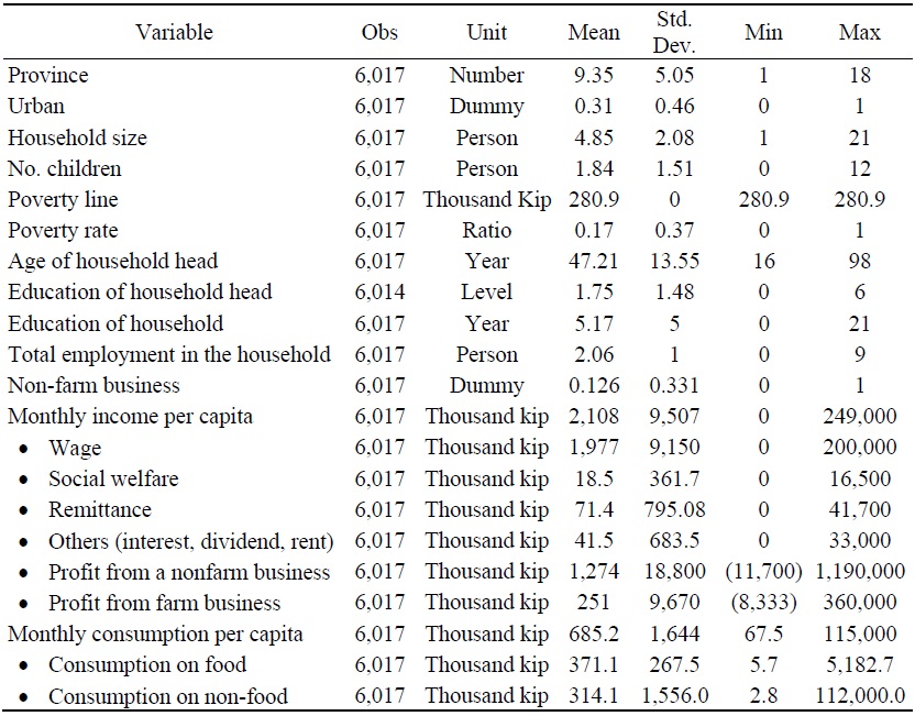
Notes: The summary statistics for household consumption on 29 food and non-food items are attached in the appendix. For education level, 0=No formal education, 1=Some primary, 2=Completed primary, 3=Completed lower secondary, 4=Completed upper secondary, 5=Completed vocational training, and 6=University degree.
Source: Author’s estimation based on LECS 6.
Figure 1.
Impact of BRI Transport via Lower Transport Cost on Changes in GDP by Region
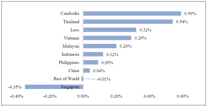
Source: Author’s estimation from using the GEMPACK economic modelling software
Table 4.
Change of Output, Employment, and Price by Sectors in Laos
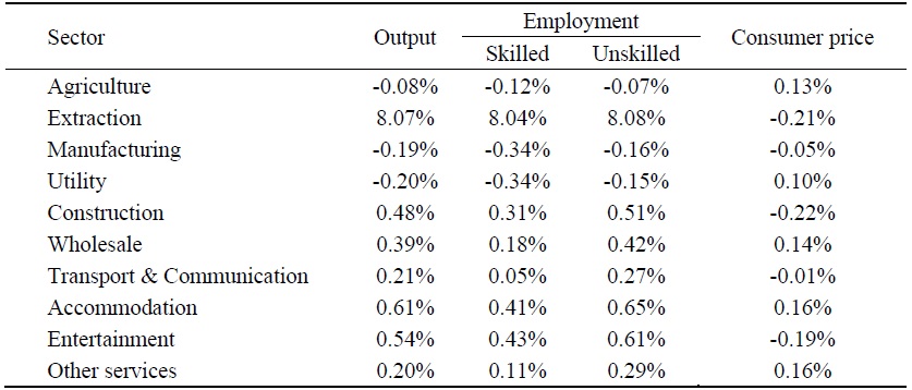
Sources: Author’s estimation from using the GEMPACK economic modelling software by
Table 5.
Impact on Poverty Reduction (%) and Income Inequality (Gini) by Regions
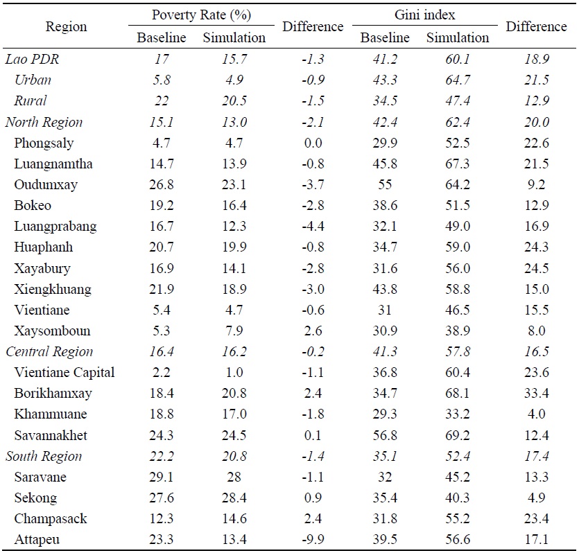
Note: The sample is 5,688 households.
Source: Author’s estimation.
Table 6.
Socioeconomics of Households in the Poverty Dynamics
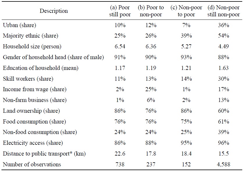
Notes: For education level, 0=No formal education,1=Some primary, 2= Completed primary, 3=Completed lower secondary, 4=Completed upper secondary, 5=Completed vocational and higher. (*) is at the village level.
Source: Authors based on LECS6.
Table 7.
Inequality Index, Income Distribution, and Income Level by Income Groups
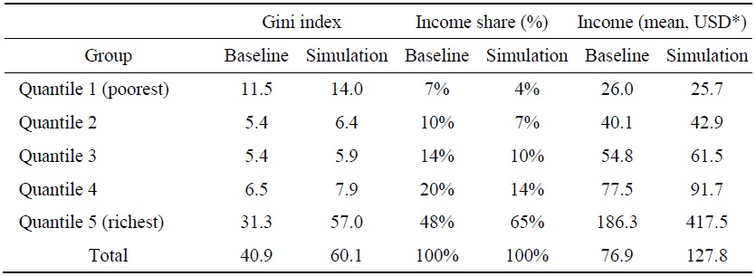
Note: (*) used the exchange rate of 8,884 Lao kip/UDS in 2019.
Source: Authors’ estimates.
Table A1.
Summary Statistics of Household’s Consumption and Budget Share in LECS6
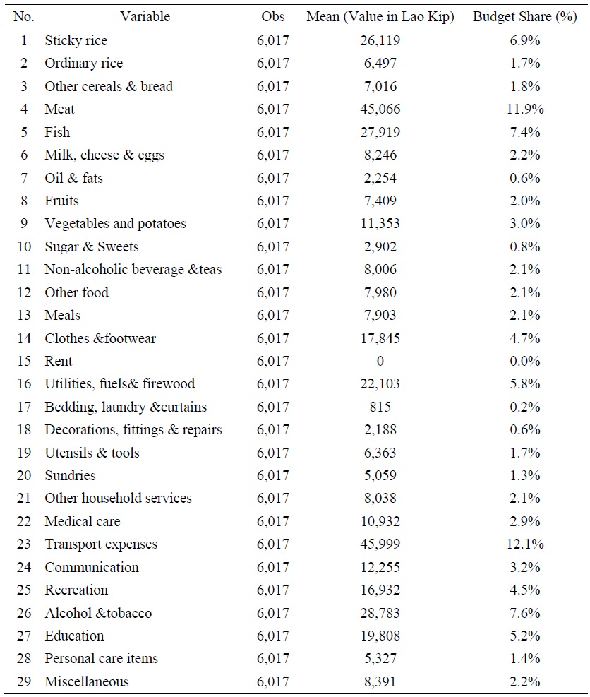
Source: Author based on LECS 6
Table A2.
Multinomial Logistic Regression: Result for Occupational Choices, Dependent Variable = Occupation
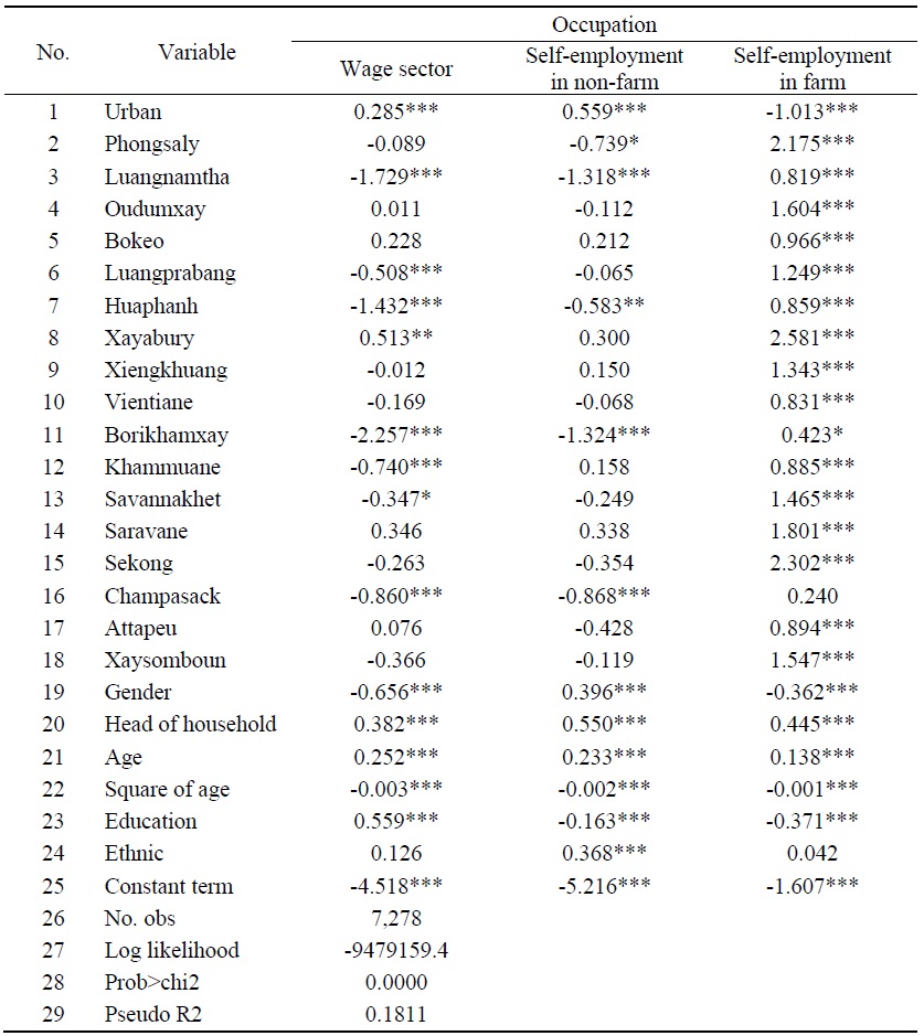
Notes: The last occupation (unemployment/not working) is the base outcome in the model. The variables of urban, provinces, gender, head of household, and ethnic are the dummy variables. For dummy variables of provinces, Vientiane capital is the based location for comparison. ***, **, and * denote significance at the 1%, 5%, and 10% level, respectively.
Source: Author’s estimation.
Table A3.
OLS Regression: Result for Business Profit Function
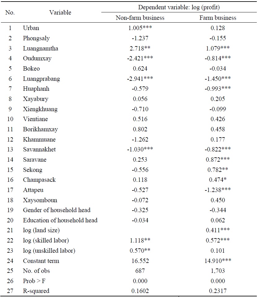
Notes: The variables of urban, provinces, and gender are the dummy variables. For dummy variables of provinces, Vientiane capital is the based location for comparison. ***, **, and * denote significance at the 1%, 5%, and 10% level, respectively.
Source: Author’s estimation.
Table A4.
GTAP Simulation Result: Impact on the Price Change of Commodities in Laos
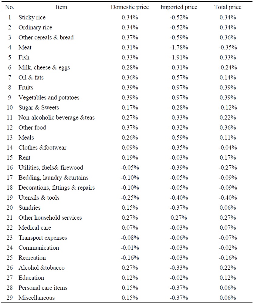
Sources: Author’s estimation from the GTAP model and GTAP database version 10. The results reported here were obtained using the GEMPACK economic modelling software by
References
-
ASEAN Secretariat. 2020.
ASEAN Key Figures 2020 . Jakarta: ASEAN Secretariat.https://www.aseanstats.org/publication/akf_2020/ -
Asian Institute of Transport Development. 2011.
Socio-economic Impact of National Highway on Rural Population (Phase II of the study). New Delhi: Asian Institute of Transport Development.http://www.aitd.net.in/pdf/studies/1.%20Socio-economic%20Impact%20of%20Nationa%20Highways%20on%20Rural%20Population%20Phase%20II.pdf -
Bandiera, L. and V. Tsiropoulos. 2020. “A Framework to Assess Debt Sustainability under the Belt and Road Initiative.”
Journal of Development Economics , vol. 146.https://doi.org/10.1016/j.jdeveco.2020.102495 
-
Bird, J., Lebrand, M. and A. J. Venables. 2020. “The Belt and Road Initiative: Reshaping economic geography in Central Asia?”
Journal of Development Economics , vol. 144.https://doi.org/10.1016/j.jdeveco.2020.102441
-
Bourguignon, F., Fournier, M. and M. Gurgand. 2001. “Fast Development with a Stable Income Distribution: Taiwan, 1979-94.”
Review of Income and Wealth , vol. 47, no. 2, pp. 139-163.https://doi.org/10.1111/1475-4991.00009
-
Burfisher, M. E. 2021.
Introduction to Computable General Equilibrium Models (3rd ed.). New York: Cambridge University Press.https://doi.org/10.1017/9781108780063 -
Cao, M. and I. Alon. 2020. “Intellectual Structure of the Belt and Road Initiative Research: A Scientometric Analysis and Suggestions for a Future Research Agenda.”
Sustainability , vol. 12, no. 17.https://doi.org/doi:10.3390/su12176901 -
Corong, E. L., Hertel, T. W., McDougall, R., Tsigas, M. E. and D. van der Mensbrugghe. 2017. “The Standard GTAP Model, Version 7.”
Journal of Global Economic Analysis , vol. 2, no. 1.https://doi.org/10.21642/JGEA.020101AF -
de Soyres, F., Mulabdic, A. and M. Ruta. 2020. “Common transport infrastructure: A quantitative model and estimates from the Belt and Road Initiative.”
Journal of Development Economics , vol. 143.https://doi.org/10.1016/j.jdeveco.2019.102415
-
Gachassin, M., Najman, B. and Raballand, G. 2010. “The Impact of Roads on Poverty Reduction: A Case Study of Cameroon.” Policy Research Working Paper, no 5209. World Bank.
http://hdl.handle.net/10986/19924 -
Ghani, E., Goswami, A. G. and W. R. Kerr. 2016. “Highway to Success: The Impact of the Golden Quadrilateral Project for the Location and Performance of Indian Manufacturing.”
Economic Journal , vol. 126, no. 591, pp. 317-357.https://dx.doi.org/10.1111/ecoj.12207
-
Gibson, J., and S. Rozelle. 2003. “Poverty and Access to Roads in Papua New Guinea.”
Economic Development and Cultural Change , vol. 52, no. 1, pp. 159-185.https://doi.org/10.1086/380424
-
Horridge, M., Jerie, M., Mustakinov, D. and F. Schiffmann. 2018. “
GEMPACK User Manual .” GEMPACK Software.https://www.copsmodels.com/gpmanual.htm -
Insisienmay, S., Sayavong, V., Thiladej, S., Vansana, P. and S. Bolivong. 2019. How to maximize the Benefits for Lao Agriculture from Regional Infrastructure Connectivity: A case study of Laos-China Railway. CMER Working paper Series, no. 0006/October 2019. Center For Macroeconomic Policy and Economic Restructuring.
https://doi.org/10.13140/RG.2.2.30121.75368 -
Kyophilavong, P., Record, R., Takamatsu, S., Nghardsaysone, K. and I. Sayvaya. 2016. “Effects of AFTA on Poverty: Evidence from Laos.”
Journal of Economic Integration , vol. 31, no. 2, pp. 353-376.
-
Lall, S. V. and M. Lebrand. 2020. “Who wins, who loses? Understanding the spatially differentiated effects of the belt and road initiative.”
Journal of Development Economics , vol. 146.https://doi.org/10.1016/j.jdeveco.2020.102496
- Lao and Chinese Government. 2017. “Master Plan of BRI Cooperation between Laos and China.” (in Lao)
- Lao and Chinese Government. 2019. “Laos-China Economic Corridor Cooperation (2019-2030) between Lao government and Chinese government.” (in Lao)
- Lao Statistics Bureau. 2012. “Growth rate of Gross Domestic Products by Industrial Origin at Constant Price 2012 [Data].” Laos Statistical Information Service (LAOSIS). (accessed December 21, 2022)
-
Lao Statistics Bureau. 2019.
Statistical Yearbook 2019 . Vientiane Capital: Lao Statistics Bureau, Ministry of Planning and Investment. -
Lao Statistics Bureau and World Bank. 2020.
Poverty Profile in Lao PDR: Poverty Report for the Lao Expenditure and Consumption Survey 2018-2019 . Vientiane Capital: Lao Statistics Bureau, Ministry of Planning and Investment. -
Lord, M. J. 2010. “Impact of the EWEC on Development in Border Provinces: Case Study of Savannakhet Province in Lao PDR.” MPRA Paper, no. 41153.
https://mpra.ub.unimuenchen.de/41153/1/MPRA_paper_41153.pdf -
Maliszewska, M. and D. van der Mensbrugghe. 2019. “The Belt and Road Initiative: Economic, Poverty and Environmental Impacts.” Policy Research Working Paper, no. 8814. World Bank.
http://hdl.handle.net/10986/31543 -
Nedopil, C. 2022. “Countries of the Belt and Road Initiative.” Green Finance & Development Center, FISF Fudan University.
https://greenfdc.org/countries-of-the-belt-and-roadinitiative-bri/ -
Tiberti, L., Cicowiez, M. and J. Cockburn. 2018. “A Top-Down with Behaviour (TDB) Microsimulation Toolkit for Distributive Analysis.”
International Journal of Microsimulation , vol. 11, no. 2, pp. 191-213.
-
United Nations. 2017. “Household Size and Composition Around the World 2017 Data Booklet.” UN Data Booklet, no. ST/ESA/SER.A/405.
https://www.un.org/development/desa/pd/content/household-size-and-composition-around-world-2017-data-booklet -
Warr, P. 2005. “Road Development and Poverty Reduction: The Case of Lao PDR.” ADB Institute Discussion Paper, no. 25. Asian Development Bank Institute.
https://www.adb.org/sites/default/files/publication/156778/adbi-dp25.pdf -
Wongpit, P. and B. Inthakesone. 2017. “Export and Import Performance of Lao’s Products.”
Southeast Asian Journal of Economics , vol. 5, no. 1, pp. 41-74. -
Zhai, F. 2018. “China’s belt and road initiative: A preliminary quantitative assessment.”
Journal of Asian Economics , vol. 55, pp. 84-92.https://doi.org/10.1016/j.asieco.2017.12.006