

- EAER>
- Journal Archive>
- Contents>
- articleView
Contents
Citation
| No | Title |
|---|
Article View
East Asian Economic Review Vol. 27, No. 3, 2023. pp. 179-211.
DOI https://dx.doi.org/10.11644/KIEP.EAER.2023.27.3.422
Number of citation : 0View
221
Download
133
Changes in Time Preference Caused by the COVID-19 Pandemic
|
|
|---|

Abstract
This paper investigates the relationship between the spread of COVID-19 and time preference. In contrast to previous studies that compared time preferences before and during the pandemic, this study estimates time preferences during the COVID-19 period using eight surveys conducted over two years. Additionally, a regression analysis was conducted on the number of new COVID-19 cases and the time elapsed since the outbreak, with estimated time preference as the dependent variable. Despite a small sample size, statistically significant results were obtained, showing that as the number of new cases increased, time preference also increased. However, this effect diminished over time and disappeared by the end of 2021 in Japan. This may be due to the public’s growing familiarity with the risks of COVID-19 and the availability of vaccines and treatments. Despite a significant increase in new cases in 2022, time preference was lower than immediately after the outbreak, and this was reflected in private investments. Immediately after the outbreak of COVID-19, private investments decreased by 12% compared to the previous year, but the investments are returning in 2022 despite the surge in the number of cases. The trend of time preference explains the trend of Japanese private investments very well.
JEL Classification: C91, D12, C11
Keywords
COVID-19 Pandemic, Time Preference, Time Discounting Factor, Marginal Effect, Bayesian Hierarchical Model
I. Introduction
The coronavirus which occurred at the end of 2019 has spread quickly around the world. In March 2020, the World Health Organization (WHO) officially declared it as a pandemic. After the long pandemic of more than two years, President Biden declared the COVID-19 pandemic “over” during an interview on September 19, 2022.1 This pandemic has brought many changes across all sectors, such as economy, education, etc. This paper investigates the changes in time preference in response to the severity of the spread of COVID-19 for over two years. Time preference is the relative valuation placed on a good at an earlier date compared with its valuation at a later date. People with high time preferences are more concerned with the needs of the present moment, whereas people with low time preferences place more importance on future needs.2 In other words, the time preference shows the degree of impatience. The changes in the rate of time preference affect both individual consumption and investment behavior because the present values are changed. Furthermore, the social discount rate is one of the important factors that determine the adoption or rejection of public projects. Therefore, it also affects national long-term plans, path of economic growth and steady-state level of a country. Investigating changes in time preference caused by the COVID-19 will be important for studying the movement of economic variables not only in Microeconomics but also in Macroeconomics.
The rate of time preference is very sensitive to changes in the economy and society. If there is a negative factor, the rate of time preference increases, and if there is a positive factor, the rate of time preference decreases. According to Phlips (1982), the rate of time preference jumped quite significantly during the Great Depression, the World Wars, and the Korean war. Cassar et al. (2017) found that the 2004 Tsunami in Thailand increased the time preference and made its victims more impatient. Ohtake et al. (2014) also showed that the painful experience of the Great East Japan Earthquake also affected the time preference. Loewenstein and Prelec (1992) and Frederick et al. (2002) are both very informative and detail-oriented on time-discounting. Matousek et al. (2022) applies a meta-analysis based on 56 researches comprising 927 estimates of the discount rate and provide a comprehensive analysis on the discount rate. Chuang and Schechter (2015) and Drichoutis and Nayga (2022) also provide details of the survey on measures of time preferences. Inferring from the previous studies, it is highly likely that the rate of time preference has been affected due to the COVID-19 pandemic.
The time preference depends not only on economic and social changes but also on individual attributes such as educational background, income, age, gender, marriage, job risk, etc. Lawrance (1991) and Harrison et al. (2002) show that poor people, elderly people, less educated people, unskilled people, people who live in town, single, etc. tend to have a higher time discount rate than people with the opposite attributes, which pertain to rich people, young people, educated people, skilled people, people who live in rural, married people, etc. Viscusi and Moore (1989) introduces the probability of death from jobs to calculate time preference in their model and shows that the death risk has a significant effect on time preference. The purpose of this research is to investigate the relationship between the degree of COVID-19 spread and the time preference during COVID-19 pandemic, not to examine the relationship between individual attributes and the time preference again. Therefore, to eliminate the effect of individual attributes on time preference as much as possible, we surveyed comparable college students in Japan. It can be said that the respondents have quite similar attributes such as age, income, area where they live, etc. Of course, it could be a problem to generalize the results of the survey conducted by one college student as the results of the whole society. Chuang and Schechter (2015) points out that many works focused on student populations lead to worries about selection and external validity. Matousek et al. (2022) mentions that it also matters whether the experiment relies on students or uses broader samples of the population. However, many previous studies use students around the world as samples and generalize the results. For example, Shefrin and Thaler (2004), Kirby (2009), Harrison et al. (2020), Snowberg and Yariv (2021), Harrison et al. (2022), etc. use students in U.S., Zeisberger et al. (2012) uses students in Germany, Drichoutis and Nayga (2022) uses students in Greece, Anderhub et al. (2001) uses students in Israel, etc.
As mentioned above, there are plenty of studies on how education level, income, age, gender, job risk, etc. affect time preferences and these relationships are so well known. Recently, researches comparing the time preference of pre-COVID-19 and the time preference of mid-COVID-19 period are also rapidly coming out. Examples include Drichoutis and Nayga (2022), Harrison et al. (2020), Angrisani et al. (2020), Zhang and Palma (2022), etc. However, few studies have investigated the relationship between the COVID-19 spread level and time preferences using longitudinal data collected during the COVID-19 pandemic, although there are some studies such as Harrison et al. (2022) and Ikeda et al. (2020) which used survey data five times during the COVID-19 pandemic. In this research, we conducted the same questionnaire survey eight times for two years during the COVID-19 pandemic, which made a regression analysis during the corona period possible, although the number of data is only eight. This is the different thing with the previous researches. We analyzed the aggregated data and estimated the time discount factor for each period from questionnaire surveys eight times. Then, by setting the estimated coefficients as a new dependent variable, a regression analysis was performed on the COVID-19 spread level and the elapsed days since the outbreak of the coronavirus. The number of data is only 8, which is very small, but we obtained statistically very significant results.
The results of the paper can be summarized as follows: (i) we found a positive relationship between the number of people newly tested positive for coronavirus and time preferences. As the number of new coronavirus infections increases, the time preference increases. The increase in the number of new coronavirus infections is considered to increase various risks in the future including the risk that people may be more likely to be infected with the coronavirus. If the future becomes unstable under the risk of coronavirus, people may reduce the importance of the uncertain future and place more importance on the present. COVID-19’s negative shocks make us impatient like other risks ? recession, war, natural disaster, etc.; (ii) we found that the effect of the number of new corona infections on time preferences was diminishing over time and eventually disappeared. It is thought that as time goes on, people become accustomed to the risk of coronavirus. Because correct information, vaccines, effective drugs, etc. have been developed for coronavirus, it is thought that the risks we feel have a lesser impact as compared to that at the beginning of the outbreak despite the increase in the number of infections. According to the results of this research, the increase in the number of new positive cases does not affect the time preferences statistically any more starting from the end of 2021. The results of previous studies have not unified the effects of the COVID-19 pandemic on the time preferences.3 For example, Gassmann et al. (2022) and Holt and Laury (2002) report that the coronavirus risk has an effect on time preference, while Lohmann et al. (2020), Harrison et al. (2020) and Harrison et al. (2022) relay that the preferences were relatively stable over the course of the pandemic. Considering the time that elapsed from the onset of corona may be one way to consistently explain this discrepancy. It can be said that the factors (i) and (ii) clarified in this research are in good agreement with intuition; (iii) we also found that time preferences for the near future are affected by the corona risk, whereas time preferences for the distant future are not. This result is deeply related to hyperbolic discounting; and (iv) in addition, the law of diminishing marginal utility for goods and the hyperbolic discount were also confirmed.
From the above results, it is thought that the influence of COVID-19 could decrease short-term investments immediately after the outbreak of COVID but the impact on long-term investments would not be so great. In fact, looking at the amount of domestic private investments in Japan, investments were about JPY 93 trillion in the third quarter in 2019 before the COVID-19 pandemic. It lowered to JPY 82 trillion in the same period in 2020, the year the pandemic was declared, causing a drop to about 11.8% compared to the previous year. However, despite the further increase in the number of infected people, the amount of investments in Japan has gradually recovered to about JPY 83 trillion in the same period in 2021 and about JPY 87 trillion in the same period in 2022.4 It is thought that this movement of investments must be closely related to the recovery of time preferences. The trend of time preference explains the trend of Japanese private investments very well.
This paper is organized as follows: Section II outlines the survey and explains how to handle the survey data; Section III reports the aggregate results of the questionnaire survey; Section IV explains the way of estimation of time discount factors and reports the estimation results and the marginal effect of the number of new infections on the time discounting factor; and Section V offers conclusions on this research. Finally, the information on estimates omitted from the body and the questionnaire used in this survey are posted in Appendix.
1)President Biden said, “We still have a problem with COVID. We’re still doing a lot of work on it. But the pandemic is over.”
2)
3)The effects of the COVID-19 pandemic on time preferences are detailed in
4)The amounts of private non-residential investment are as follows: 93,329.80 from Jul/2019 to Sep/2019, 82,306.20 from Jul/2020 to Sep/2020, 83,099.10 from Jul/2021 to Sep/2021, 86,563.80 from Jul/2022 to Sep/2022 (Unit: Billions of 2015 Chained Yen). See Cabinet Office Japan,
II. Outline of Survey
1. The Survey
Questionnaires and experiments are becoming common methods in research on time preferences. We used a questionnaire that was almost the same as the one employed in Shin (2021). While Shin (2021) focused on exploring hyperbolic discounting and magnitude effects in the field of behavioral economics, this research aimed to investigate changes in discount rates during the COVID-19 pandemic. In this research, a survey was conducted among students at Asia University in Tokyo, Japan using a questionnaire that was originally developed. The survey lasted for 2 years from July 2020 to July 2022. It was carried out eight times using the same questionnaire to investigate the relationship between the severity of the COVID-19 situation and time preference. We collected the responses via a website in light of the difficulty of data collection if it were to be done on paper. The questionnaire was posted on a website and disseminated during the classes that the author of this research teaches. Students participated at any time during the survey period.
Table 1 summarizes the detailed survey schedule, the number of respondents, the number of new coronavirus infections in Tokyo, and the number of elapsed days. The number of elapsed days is arrived at using the mean of the periods. Assume that January 1, 2020 is day 1, January 2, 2020 is day 2, and so forth. Accordingly, September 19, 2022, is counted as 993. In the case of the first period, which is from 7/19/2020 to 8/7/2020, the mean is computed as 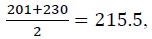 and in the case of the second period, which is from 12/6/2020 to 12/26/2020, the mean is
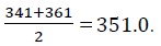
Figure 1 visually shows the number of respondents and the number of new coronavirus infections in Tokyo. The horizontal axis represents the elapsed days. The left vertical axis represents the number of new coronavirus infections in Tokyo, and the right vertical axis represents the number of respondents to the survey.
Responses were obtained from freshmen (1st year student) to seniors (4th year student). In light with preserving the privacy of the respondents and in keeping the research free from all prejudice and bias, the concerns of the respondents, the response rate, and any data with regard to the respondents’ personal information, such as name, grade, gender, income, etc., are kept anonymous. The questionnaire used in this research is attached in the Appendix B. This is a selection questionnaire, not a descriptive survey, where the combinations of the amount of money received and the timing are used. We prepared four kinds of money to be received: 10,000 yen, 30,000 yen, 50,000 yen, and 100,000 yen, and five kinds of reception timing: Today, 3 months later, 6 months later, 12 months later, and 36 months later. The number of combinations between the money and timing was 60. The questions are in a two-choice format. For example:
Please, choose between the two scenarios.
○ get 10,000 yen only for today
○ get 30,000 yen if you wait for 3 months
Please, choose between the two scenarios.
○ get 10,000 yen only for today
○ get 50,000 yen if you wait for 3 months
The questionnaire used in the survey does not have question numbers (e.g., Q3, Q4). However, for ease of explanation, the question numbers have been assigned herein. The number of questions in the two-choice format was 60. The correspondents do not need to answer every single one of the 60 questions completely. Respondents’ answers to related questions are predictable. For example, we can expect easily that if the correspondents choose the second option from Q3 then they will choose the second option from Q4. So, we don’t ask them Q4 and they don’t need to answer it. In the case that the correspondents choose the second option from Q6, we don’t ask them Q9, Q12 and Q14 because we can anticipate them choosing the first option in the proceeding questions. As stated by these examples, the questions are different according to the choices the correspondents pick. The correspondents answered only about 30 questions on average from the 60 questions.
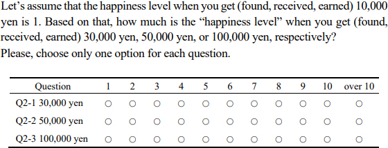
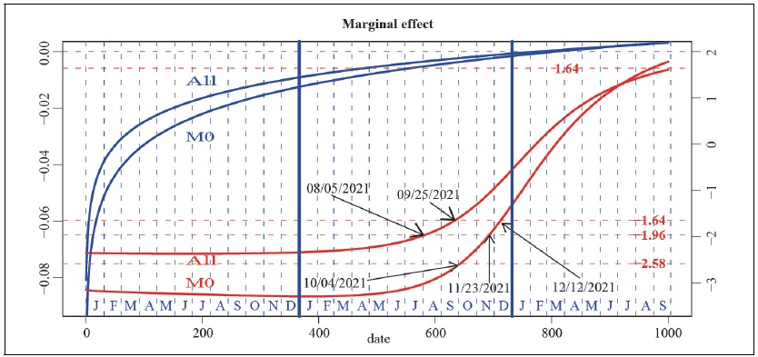
We also asked about their happiness level with the amount they received. We prepared eleven choices – 1, 2, 3, ⋯, 9, 10 and over 10 – for the happiness level when they receive the money, 1 being the lowest. The questions are below.
Research on time preference is a well-established field with a long history of estimation. Renowned research papers, such as Andersen et al. (2008) and Andreoni and Sprenger (2012), have significantly contributed to this area by utilizing the CRRA (Constant Relative Risk Aversion) utility function as a theoretical foundation to estimate risk and discount rates. In this paper, we adopt a straightforward approach by using surveys to directly inquire about happiness levels and employ this information to estimate discount rates. Due to the qualitative nature of happiness levels, obtaining precise responses can be challenging, leading to a higher frequency of unusual answers compared to estimation methods that assume utility functions.5 Nevertheless, this research opts for the direct and simple method of questioning happiness levels.
2. Worrisome Data and Handling
It is difficult to quantify the happiness level related to money from option “over 10.” Therefore, for the sake of convenience, we omitted them from our analysis. Of the total 2,785 samples, 1,907 samples (68.5%) were used for analysis, excluding 878 samples (31.5%) who selected “over 10.” The possibility of selection bias cannot be excluded from the analysis results of this study. A research on the information of “over 10” is a future topic. The number of samples listed in Table 1 excludes the answers of students who chose “over 10.”
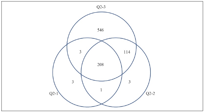
There were 215, 326 and 871 respondents who answered “over 10” to Q2-1, Q2-2 and Q2-3, respectively. It seems appropriate that the higher the amount they receive, the larger the number of respondents who answered “over 10.” 209 respondents answered “over 10” for both Q2-1 and Q2-2. 211 respondents answered “over 10” for both Q2-1 and Q2-3. 322 respondents answered “over 10” for both Q2-2 and Q2-3. 208 respondents answered “over 10” for all of Q2-1, Q2-2 and Q2-3. The numbers of students who chose “over 10” are summarized in the Venn diagram in Figure 2. Three students answered “over 10” for Q2-1 and answered under 10 for Q2-2 and Q2-3. The happiness of receiving 10,000 yen was greater than the happiness of receiving 30,000 yen and 50,000 yen. It is a little weird. At this point, some respondents may have taken the survey lightly.
Of the 1,907 students, 76 students chose option 1 for Q2-1, Q2-2, and Q2-3, 20 students chose option 2 in all questions, 24 students chose option 3, 58 students chose option 4, 26 students chose option 5, 0 students chose option 6, 2 students chose option 7, 2 students chose option 8, 3 students chose option 9, and 34 students chose option 10. They (245 students) were equally satisfied when they received 30,000 yen or 50,000 yen or 100,000 yen. It is also a little weird. We can consider several reasons, among others: (1) As the marginal utility of money decreases, the marginal utility would approach almost zero, then their utility level is almost the same even though the money they receive increases; or (2) The students already knew the scenarios to be fictional (they do not get the money for real), so they did not answer seriously and so on. The results have been derived from the students’ own discretion arbitrarily or whimsically; or (3) Matousek et al. (2002) found that that real or hypothetical payoffs for discounting experiments do not make a difference. Hence, the issues may be the result of a lack of incentivization; or for various other reasons which remain unknown. It may be challenging for anyone other than the survey respondents to ascertain this point. We used their data for analysis without making any subjective judgments about it.6
5)The occurrence of worrisome results in Section II.2 could be one of the reasons for this.
6)We present the facts objectively and without bias and leave the judgment about this issue to the reader.
III. The Descriptive Statistics for the Survey
1. Q3 to Q62
We assigned the code 0 for those who chose the first one which opts for earlier receipt, and 1 for those who chose the second one for late receipt. Table 2 shows the question numbers with the highest number of respondents choosing options 0 and 1, the number of respondents and their ratio. The question with the highest number of respondents who chose option 0 was Q11. The respondents are 1,598 (83.8 %). Q11 is as follows:
Please, choose between the two scenarios.
○ get 10,000 yen only for today
○ get 30,000 yen if you wait for 36 months (3 years)
On the other hand, the question with the highest number of respondents who chose option 1, was Q30. The respondents are 1,793 (94.0%). Q30 is as follows:
Please, choose between the two scenarios.
○ get 10,000 yen if you wait for 3 months
○ get 100,000 yen if you wait for 6 months
In Q11, the first option “10,000 yen Today” is compared to the second option “30,000 yen 36 months later” which is deemed the worst condition among the combinations because it has the longest period (36 months) for the least amount (30,000 yen) to be received. Therefore, it is thought that many students chose the first option “10,000 yen Today”. On the other hand, in Q30, the first option “10,000 yen 3 months later” is compared to the second option “100,000 yen 6 months later” which is deemed the best condition among the combinations because it has only 3 months for the largest amount (100,000 yen) to be received. Therefore, it is thought that many students chose the second option “100,000 yen 6 months later”. Q21 and Q6 can be explained in almost the same way.7 This result makes a lot of sense. From these results, the answers to this questionnaire survey are considered to be quite reliable. Moreover, the results in Table 2 show a significant alignment with the findings of the survey conducted before the COVID-19 period, as presented in Shin (2021). This indicates a certain degree of survey robustness.
We aggregated the answers of Q2. Table 3 summarizes the happiness level for 30,000 yen, 50,000 yen, and 100,000 yen and the marginal happiness. H30,000, H50,000, and H100,000 are the happiness level when receiving 30,000 yen, 50,000 yen, and 100,000 yen, respectively. MH1 represents marginal happiness in money between 10,000 yen and 30,000 yen, MH2 represents marginal happiness in money between 30,000 yen and 50,000 yen, and MH3 represents marginal happiness in money between 50,000 yen and 100,000 yen. We calculate the arithmetic means of the values chosen by the respondents for each period. As seen in Section II, for some students (245 students), the levels of happiness were equal even though the amount received increased, however, it was found that for the average of the whole sample, in all eight periods, the higher the amount received was, the higher the happiness level was as shown in Table 3 (e.g., 3.225 < 4.424 < 6.437). As the money they receive increases, the marginal happiness decreases in all eight periods (e.g., MH1 (1.112) > MH2 (0.600) > MH3 (0.403)). We can imagine that the curve of happiness level is not linear, but becomes flattered as the money increases, that is, the marginal happiness level for money gradually decreases as shown in normal goods.
7)Considering the “hyperbolic discount,” it is understandable that the lowest is Q30, not Q6.
IV. Time Discounting Factor
1. Estimation Model
In this paper, we use happiness level (utility level) to try to estimate the rate of time discount factor.8 We estimate the discount factor for the duration of 8 questionnaires and the entire period.9 When the discount factor is low, the weight for future happiness is small. In other words, the future happiness is greatly discounted. Conversely, when the discount factor is high, the weight for future happiness is large. In other words, it does not discount much future happiness.
Let us define the exponential discount function (
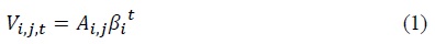
where,
We consider a function of softmax action selection (
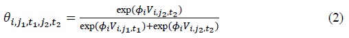
where,

There are two kinds of parameters –
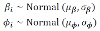
where, 

 where
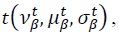
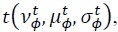
where  are parameters (or arguments) required for the distribution functions. These parameters are specified to make the hyperprior vague as follows:

The estimation was performed using the Bayesian hierarchical model. The sampling was run with a burn-in of 2,000 iterations out of the 10,000 iterations and with 4 chains. The estimated results of
2. Estimation Results of Time Discount Factor
Table 4 summarizes the estimated
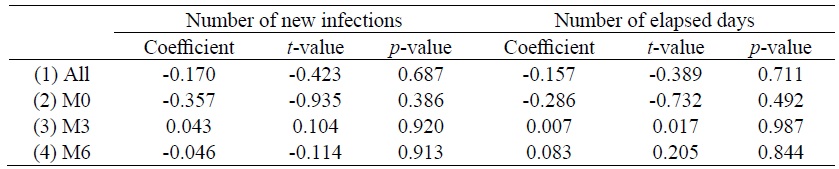
3. Correlation and Regression Analysis
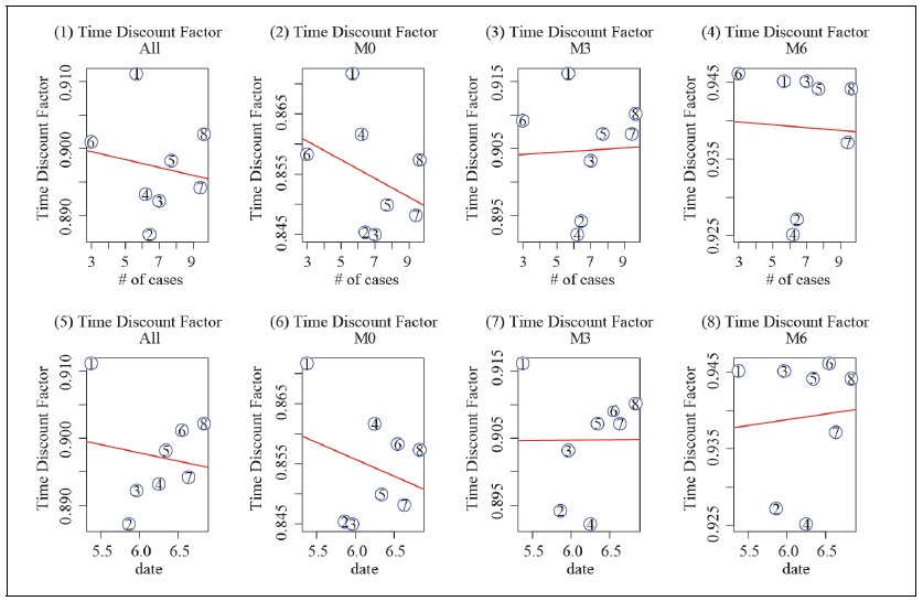
To investigate the relationship between the number of new infections and the time-discounting factor, and the relationship between the number of days elapsed and the time-discounting factor, we plot the data on Figure 3. The horizontal axes of (1)-(4) show the number of newly infected people, and the horizontal axes of (5)-(8) show the number of days elapsed. The vertical axes show the time discount factor. The number in the circle represents the period in which the surveys were conducted. The red lines are the regression lines when the estimated time discount factors (
It is thought that there is more complex relationship between the time discount actor and the number of new infections and the elapsed time, not just a simple correlation. We performed a multiple regression analysis that considers the number of newly infected people, the elapsed date and their product such as Equation (4). The estimated time discount factor in Table 4 were used as dependent variables.11

where,
When the dependent variable was set to the time discount factor in the column (1) All and (2) M0,
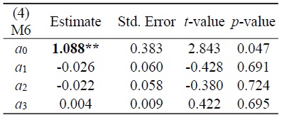
4. Marginal Effect of COVID-19
We will focus on the case where the dependent variables are set to (1) All and (2) M0 where
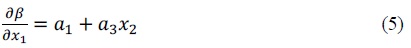
If the value of Equation (5) is positive  the number of infected people has a positive effect on the time discount factor. Oppositely, if the value of Equation (5) is negative
  the number of infected people has a negative effect on the time discount factor. According to the estimation results, because
The marginal effects of coronavirus on the time discount factor and the
The marginal effect of the number of new infections on the time discount factor immediately after the outbreak of the coronavirus is large, but the effect gradually decreases and eventually disappears. Since the end of 2021, the marginal effect of the number of new infections is no longer significant. Because of the development of vaccines and effective drugs and the weakening of the virus itself, people have become accustomed to the dangers of COVID-19. Therefore, it is thought that the discount rate at the time of the COVID-19 outbreak is returning to its original level. In the case of the 8th period, although the number of new infections was the highest, the time discount was low.
Ohtake et al. (2014) conducted a survey two years after the tsunami. The author reports that the risk of the Great East Japan Earthquake still affects time preferences after two years. In this study, the effect of COVID-19 on the time discount factor was not continued for more than two years. In the case of natural disasters such as tsunamis and earthquakes, it is difficult to predict the timing of recurrence, so the magnitude of the risk is difficult to predict. However, in the case of COVID-19, new outbreaks were reported every day, and the degree of risk was somewhat predictable. In this respect, it can be predicted that the duration of COVID-19 effect on the time preference rate was shorter than that of the tsunami’s effect. In addition, in the case of the tsunami, the survey was conducted only on Tohoku residents who suffered damage, while this study was conducted on both students who were infected and uninfected, so the negative impact of the corona may have been shorter than that of the tsunami.
8)We used the same discount rate estimation method as
9)There is the relationship between the time-discounting rate ( The relationship between discount rate and time preference is shown as the discount rate=time preference+1 in
10)In Behavioral Economics, “hyperbolic discount” and “magnitude effect” are among well-known factors on the time-discounting rate: (i) “hyperbolic discount” (also known as “present bias”) suggests that values placed on rewards decrease very rapidly for small delay periods and then fall more slowly for longer delays
11)A measurement error may also occur if the orthogonality condition between the error term of the time discounting factor and the explanatory variables is not satisfied.
12)When the dependent variable is (1) All, 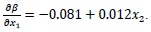 When
When 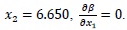 When the dependent variable is (2) M0,
  When
When  Converting these values to elapsed days, in case of (1) All, exp(6.650) = 773, then February 11, 2022, in case of (2) M0, exp(6.693) = 807, then March 17, 2022.
V. Conclusion
More than two years have passed since the start of the coronavirus until President Biden declared the COVID-19 pandemic “over,” and it has brought about huge changes in our lives. In this research, we investigated the relationship between the spread of COVID-19 and time preferences. Time preferences are very important in that they provide a guide not only for individual consumption and investment, but also for macroeconomic policies.
In this paper, we conducted a questionnaire survey on college students in Tokyo Japan. There are a lot of studies on the time-discounting rate by using questionnaire surveys which compare pre-corona and mid-corona periods. However, few studies have investigated the relationship between COVID-19 expansion status and time preference during mid-COVID-19 pandemic using longitudinal data collected during its prevalence. We conducted surveys eight times during the COVID-19 pandemic period, collected the longitudinal data and estimated the time preference for the COVID-19 expansion situation. Then, the estimated values were used as the dependent variables. Despite the small amount of data, highly statistically significant results were obtained.
In this survey, we confirmed a positive relationship between the number of new corona infections and the time preference. However, the effect weakens with time and eventually disappears. Since the end of 2021, the increase in the number of new positives did not affect time preferences any more, statistically, because correct information, vaccines, and effective drugs for corona have been developed. Even though the number of infected people increased in 2022, it is thought that the perceived risk decreased compared to the beginning of the corona outbreak. In consideration of elapsed time and hyperbolic discounting, we also found that near-future time preferences are affected by corona risk, whereas distant-future time preferences are not. The separation of near-future time preferences and distant-future time preferences may resolve the inconsistent results of previous studies on the COVID-19.
The COVID-19 pandemic may have reduced short-term investments, but does not majorly affect long-term investments. The amount of domestic private investments in Japan decreased immediately after the outbreak of the coronavirus, but after that, despite the worsening condition of the corona situation, it has been returning little by little. It can be judged that there is a deep relationship with the return of time preference. In addition, we also found the marginal utility of money diminishing just as with general economic goods (also known as Gossen’s law) and hyperbolic discounting.
The analysis in this research has some problems, such as the generalization of the results from the sample collected from college students to the entire economy, the elimination of option “over 10,” the lack of incentivization, and the analysis based on the eight samples. Considering these factors remains to be seen in our future research.
Tables & Figures
Table 1.
Survey and the Number of People New Tested Positive in Tokyo
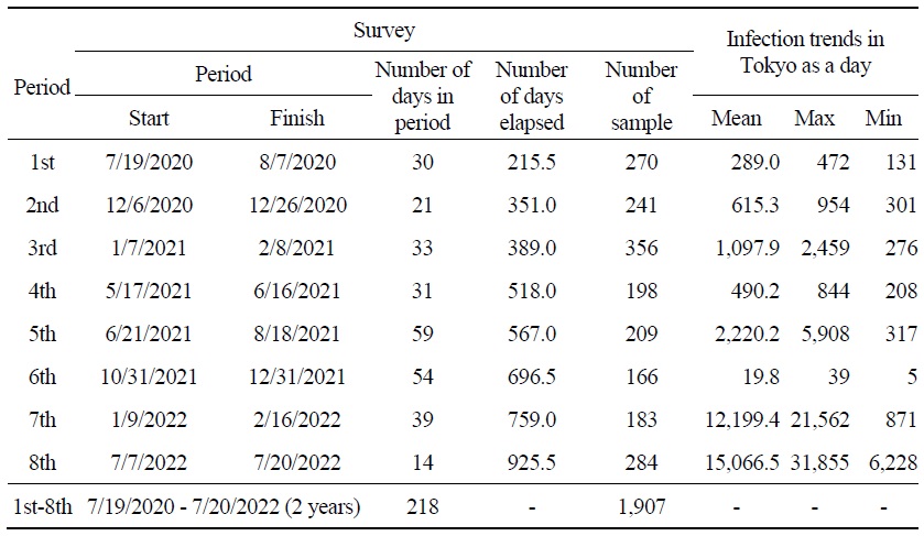
Figure 1.
The Number of Respondents to the Survey and the Number of People New Tested Positive in Tokyo
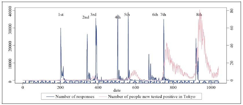
Source: COVID-19 Information Website, Tokyo Metropolitan Government.
Figure 2.
Venn Diagram for “over 10”
Source: Created by the author.
Table 2.
The Highest Answered Questions
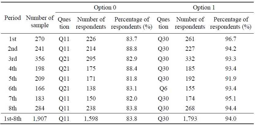
Table 3.
Happiness Level and Marginal Happiness for Money
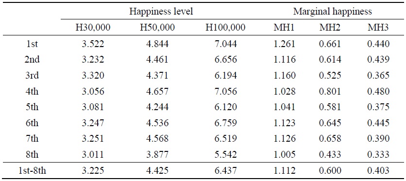
Table 4.
Estimation Results of Time Discount Factor
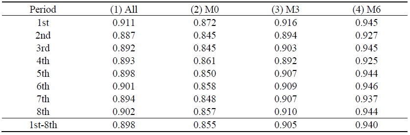
Figure 3.
Discount Rate
Source: Created by the author.
Table 5.
Correlation Coefficient
Note: All correlation coefficients are not significant at the 5% level.
Table 6.
When the Dependent Variable is (1) All
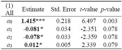
Notes: Significant codes: *** (
R-squared: 0.594, Adjusted R-squared: 0.290
Table 7.
When the Dependent Variable is (2) M0
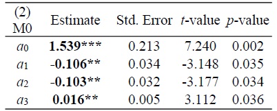
Notes: Significant codes: *** (
R-squared: 0.753, Adjusted R-squared: 0.567
Table 8.
When the Dependent Variable is (3) M3
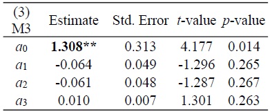
Notes: Significant codes: ** (
R-squared: 0.299, Adjusted R-squared: -0.227
Table 9.
When the Dependent Variable is (4) M6
Notes: Significant codes: ** (
R-squared: 0.06, Adjusted R-squared: -0.652
Figure 4.
Marginal Effect of the Number of Newly Infected People on Time Discounting Factor
Source: Created by the author.
APPENDIX A
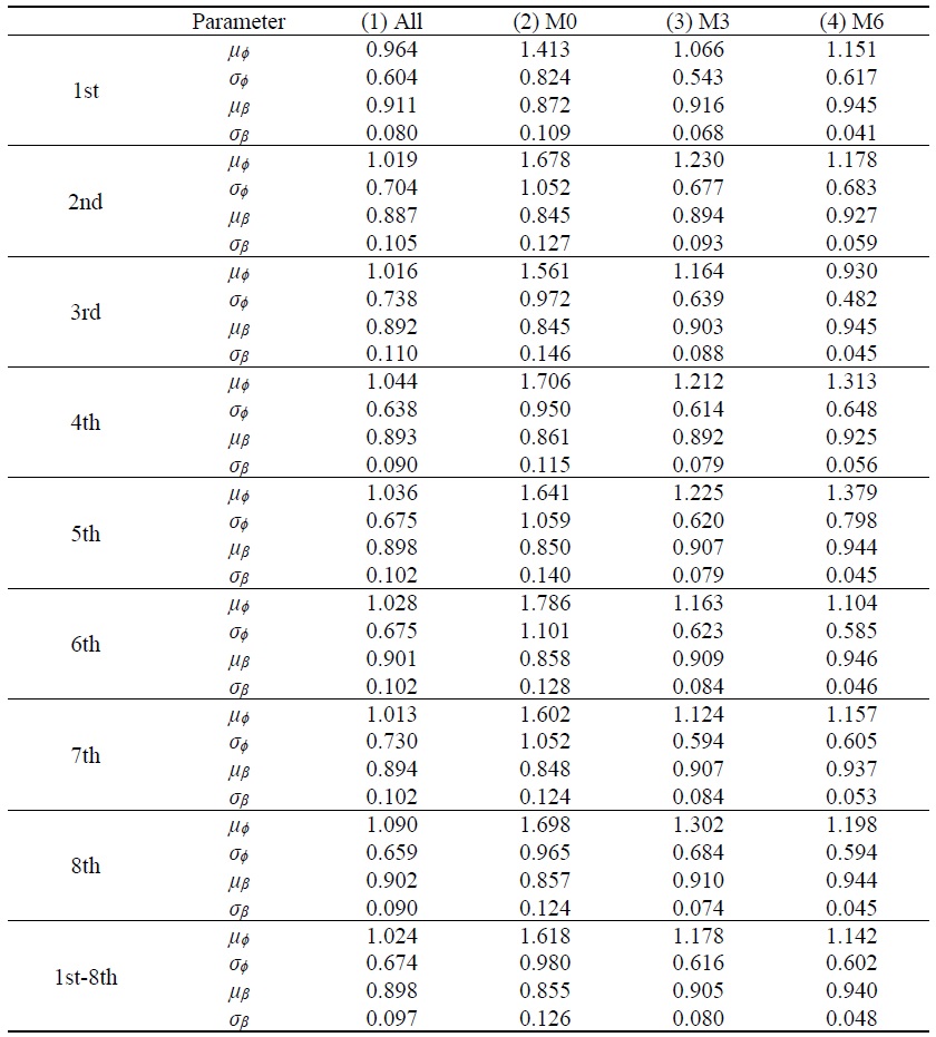
We report the estimation results of
APPENDIX B: The questionnaire
This is a survey for a research on “Discount of Money”. There are no right or wrong answers. Your responses are anonymous and confidential. No personal name or contact information is collected. However, if you want to know the results of my research, please, put your name and e-mail address on the last page. I will send the results when I finish this research.
There are 63 questions in this questionnaire, however, the correspondents will answer only about 30 questions. The questions are different according to what choice you pick. Don’t take this survey seriously.
Thank you very much for your cooperation.
Let’s assume that the happiness level when you get (found, received, earned) 10,000 yen is 1. Based on that, how much is the “happiness level” when you get (found, received, earned) 30,000 yen, 50,000 yen, or 100,000 yen, respectively?
Please, choose only one option for each question.
Please, choose between the two scenarios.
○ get 10,000 yen only for today
○ get 30,000 yen if you wait for 3 months
Please, choose between the two scenarios.
○ get 10,000 yen only for today
○ get 50,000 yen if you wait for 3 months
Please, choose between the two scenarios.
○ get 10,000 yen only for today
○ get 30,000 yen if you wait for 6 months
Please, choose between the two scenarios.
○ get 10,000 yen only for today
○ get 100,000 yen if you wait for 3 months
Please, choose between the two scenarios.
○ get 10,000 yen only for today
○ get 50,000 yen if you wait for 6 months
Please, choose between the two scenarios.
○ get 10,000 yen only for today
○ get 30,000 yen if you wait for 12 months (1 year)
Please, choose between the two scenarios.
○ get 10,000 yen only for today
○ get 100,000 yen if you wait for 6 months
Please, choose between the two scenarios.
○ get 10,000 yen only for today
○ get 50,000 yen if you wait for 12 months (1 year)
Please, choose between the two scenarios.
○ get 10,000 yen only for today
○ get 30,000 yen if you wait for 36 months (3 years)
Please, choose between the two scenarios.
○ get 10,000 yen only for today
○ get 100,000 yen if you wait for 12 months (1 year)
Please, choose between the two scenarios.
○ get 10,000 yen only for today
○ get 50,000 yen if you wait for 36 months (3 years)
Please, choose between the two scenarios.
○ get 10,000 yen only for today
○ get 100,000 yen if you wait for 36 months (3 years)
Please, choose between the two scenarios.
○ get 30,000 yen only for today
○ get 50,000 yen if you wait for 3 months
Please, choose between the two scenarios.
○ get 30,000 yen only for today
○ get 100,000 yen if you wait for 3 months
Please, choose between the two scenarios.
○ get 30,000 yen only for today
○ get 50,000 yen if you wait for 6 months
Please, choose between the two scenarios.
○ get 30,000 yen only for today
○ get 100,000 yen if you wait for 6 months
Please, choose between the two scenarios.
○ get 30,000 yen only for today
○ get 50,000 yen if you wait for 12 months (1 year)
Please, choose between the two scenarios.
○ get 30,000 yen only for today
○ get 100,000 yen if you wait for 12 months (1 year)
Please, choose between the two scenarios.
○ get 30,000 yen only for today
○ get 50,000 yen if you wait for 36 months (3 years)
Please, choose between the two scenarios.
○ get 30,000 yen only for today
○ get 100,000 yen if you wait for 36 months (3 years)
Please, choose between the two scenarios.
○ get 50,000 yen only for today
○ get 100,000 yen if you wait for 3 months
Please, choose between the two scenarios.
○ get 50,000 yen only for today
○ get 100,000 yen if you wait for 6 months
Please, choose between the two scenarios.
○ get 50,000 yen only for today
○ get 100,000 yen if you wait for 12 months (1 year)
Please, choose between the two scenarios.
○ get 50,000 yen only for today
○ get 100,000 yen if you wait for 36 months (3 years)
Please, choose between the two scenarios.
○ get 10,000 yen if you wait for 3 months
○ get 30,000 yen if you wait for 6 months
Please, choose between the two scenarios.
○ get 10,000 yen if you wait for 3 months
○ get 50,000 yen if you wait for 6 months
Please, choose between the two scenarios.
○ get 10,000 yen if you wait for 3 months
○ get 30,000 yen if you wait for 12 months (1 year)
Please, choose between the two scenarios.
○ get 10,000 yen if you wait for 3 months
○ get 100,000 yen if you wait for 6 months
Please, choose between the two scenarios.
○ get 10,000 yen if you wait for 3 months
○ get 50,000 yen if you wait for 12 months (1 year)
Please, choose between the two scenarios.
○ get 10,000 yen if you wait for 3 months
○ get 30,000 yen if you wait for 36 months (3 years)
Please, choose between the two scenarios.
○ get 10,000 yen if you wait for 3 months
○ get 100,000 yen if you wait for 12 months (1 year)
Please, choose between the two scenarios.
○ get 10,000 yen if you wait for 3 months
○ get 50,000 yen if you wait for 36 months (3 years)
Please, choose between the two scenarios.
○ get 10,000 yen if you wait for 3 months
○ get 100,000 yen if you wait for 36 months (3 years)
Please, choose between the two scenarios.
○ get 30,000 yen if you wait for 3 months
○ get 50,000 yen if you wait for 6 months
Please, choose between the two scenarios.
○ get 30,000 yen if you wait for 3 months
○ get 100,000 yen if you wait for 6 months
Please, choose between the two scenarios.
○ get 30,000 yen if you wait for 3 months
○ get 50,000 yen if you wait for 12 months (1 year)
Please, choose between the two scenarios.
○ get 30,000 yen if you wait for 3 months
○ get 100,000 yen if you wait for 12 months (1 year)
Please, choose between the two scenarios.
○ get 30,000 yen if you wait for 3 months
○ get 50,000 yen if you wait for 36 months (3 years)
Please, choose between the two scenarios.
○ get 30,000 yen if you wait for 3 months
○ get 100,000 yen if you wait for 36 months (3 years)
Please, choose between the two scenarios.
○ get 50,000 yen if you wait for 3 months
○ get 100,000 yen if you wait for 6 months
Please, choose between the two scenarios.
○ get 50,000 yen if you wait for 3 months
○ get 100,000 yen if you wait for 12 months (1 year)
Please, choose between the two scenarios.
○ get 50,000 yen if you wait for 3 months
○ get 100,000 yen if you wait for 36 months (3 years)
Please, choose between the two scenarios.
○ get 10,000 yen if you wait for 6 months
○ get 30,000 yen if you wait for 12 months (1 year)
Please, choose between the two scenarios.
○ get 10,000 yen if you wait for 6 months
○ get 50,000 yen if you wait for 12 months (1 year)
Please, choose between the two scenarios.
○ get 10,000 yen if you wait for 6 months
○ get 30,000 yen if you wait for 36 months (3 years)
Please, choose between the two scenarios.
○ get 10,000 yen if you wait for 6 months
○ get 100,000 yen if you wait for 12 months (1 year)
Please, choose between the two scenarios.
○ get 10,000 yen if you wait for 6 months
○ get 50,000 yen if you wait for 36 months (3 years)
Please, choose between the two scenarios.
○ get 10,000 yen if you wait for 6 months
○ get 100,000 yen if you wait for 36 months (3 years)
Please, choose between the two scenarios.
○ get 30,000 yen if you wait for 6 months
○ get 50,000 yen if you wait for 12 months (1 year)
Please, choose between the two scenarios.
○ get 30,000 yen if you wait for 6 months
○ get 100,000 yen if you wait for 12 months (1 year)
Please, choose between the two scenarios.
○ get 30,000 yen if you wait for 6 months
○ get 50,000 yen if you wait for 36 months (3 years)
Please, choose between the two scenarios.
○ get 30,000 yen if you wait for 6 months
○ get 100,000 yen if you wait for 36 months (3 years)
Please, choose between the two scenarios.
○ get 50,000 yen if you wait for 6 months
○ get 100,000 yen if you wait for 12 months (1 year)
Please, choose between the two scenarios.
○ get 50,000 yen if you wait for 6 months
○ get 100,000 yen if you wait for 36 months (3 years)
Please, choose between the two scenarios.
○ get 10,000 yen if you wait for 12 months (1 year)
○ get 30,000 yen if you wait for 36 months (3 years)
Please, choose between the two scenarios.
○ get 10,000 yen if you wait for 12 months (1 year)
○ get 50,000 yen if you wait for 36 months (3 years)
Please, choose between the two scenarios.
○ get 10,000 yen if you wait for 12 months (1 year)
○ get 100,000 yen if you wait for 36 months (3 years)
Please, choose between the two scenarios.
○ get 30,000 yen if you wait for 12 months (1 year)
○ get 50,000 yen if you wait for 36 months (3 years)
Please, choose between the two scenarios.
○ get 30,000 yen if you wait for 12 months (1 year)
○ get 100,000 yen if you wait for 36 months (3 years)
Please, choose between the two scenarios.
○ get 50,000 yen if you wait for 12 months (1 year)
○ get 100,000 yen if you wait for 36 months (3 years)
If you want to know the results of my research, please, put your name and e-mail address on the blanks. I will send the results when I finish this research.
name:
e-mail address:
Appendix Tables & Figures
Table A1.
Estimation Results
References
-
Anderhub, V., Guth, W., Gneezy, U. and D. Sonsino. 2001. “On the Interaction of Risk and Time Preference: An Experimental Study.”
German Economic Review , vol. 2, no. 3, pp. 239-253.
-
Andersen, S., Harrison, G., Lau, M. and E. Rutstrom. 2008. “Eliciting Risk and Time Preferences.”
Econometrica , vol. 76, no. 3, pp. 583-618.
-
Andreoni, J. and C. Sprenger. 2012. “Estimating Time Preferences from Convex Budgets.”
American Economic Review , vol. 102, no. 7, pp. 3333-3356.
- Angrisani, M., Cipriani, M., Guarino, A., Kendall, R. and J. Ortiz de Zarate Pina. 2020. “Risk Preferences at the Time of COVID-19: An Experiment with Professional Traders and Students.” FRBNY Staff Report, no. 927. Federal Reserve Bank of New York.
-
Benzion, U., Rapaport, A. and J. Yagil. 1989. “Discount Rates Inferred from Decisions: An Experimental Study.”
Management Science , vol. 35, no. 3, pp. 270-284.
-
Cassar, A., Healy, A. and C. von Kessler. 2017. “Trust, Risk, and Time Preferences After a Natural Disaster: Experimental Evidence from Thailand.”
World Development , vol. 94, pp. 90-105.
-
Chuang, Y. and L. Schechter. 2015. “Stability of experimental and survey measures of risk, time, and social preferences: A review and some new results.”
Journal of Development Economics , vol. 117, pp. 151-170.
-
Drichoutis, A. and R. M. Nayga. 2022. “On the stability of risk and time preferences amid the COVID-19 pandemic.”
Experimental Economics , vol. 25, pp. 759-794.https://doi.org/10.1007/s10683-021-09727-6
-
Frederick, S., Loewenstein, G. and T. O’Donoghue. 2002. “Time Discounting and Time Preference: A Critical Review.”
Journal of Economic Literature , vol. 40, no. 2, pp. 351-401.
-
Frey, B. 2008. Happiness: A revolution in economics. Cambridge, MA: MIT Press.
https://doi.org/10.7551/mitpress/9780262062770.001.0001 -
Gassmann, X., Malezieux, A., Spiegelman, E. and J.-C. Tisserand. 2022. “Preferences after pandemics: Time and risk in the shadow of COVID-19.”
Judgment and Decision Making , vol. 17, no. 4, pp. 745-767.
-
Gelman, A. and D. B. Rubin. 1992. “Inference from Iterative Simulation Using Multiple Sequences.”
Statistical Science , vol. 7, no. 4, pp. 457-472. -
Green, L., Myerson, J. and E. McFadden. 1997. “Rate of Temporal Discounting Decreases with Amount of Reward.”
Memory and Cognition , vol. 25, no. 5, pp. 715-723.https://doi.org/10.3758/BF03211314
-
Harrison, G. W., Hofmeyr, A., Kincaid, H., Monroe, B., Ross, D., Schneider, M. and J. T. Swarthout. 2022. “Subjective beliefs and economic preferences during the COVID-19 pandemic.”
Experimental Economics , vol. 25, no. 3, pp. 795-823.https://doi.org/10.1007/s10683-021-09738-3
-
Harrison, G. W., Lau, M. I. and M. B. Williams. 2002. “Estimating Individual Discount Rates in Denmark: A Field Experiment.”
American Economic Review , vol. 92, no. 5, pp. 1606-1617.http://www.doi.org/10.1257/000282802762024674
-
Harrison, G. W., Lau, M. I. and H. I. Yoo. 2020. “Risk Attitudes, Sample Selection and Attrition in a Longitudinal Field Experiment.”
Review of Economics and Statistics , vol. 102, no. 3, pp. 552-568.
-
Holt, C. A. and S. K. Laury. 2002. “Risk aversion and incentive effects.”
American Economic Review , vol. 92, no. 5, pp.1644-1655.https://doi.org/10.1257/000282802762024700
-
Ikeda, S., Yamamura, E. and Y. Tsutsui. 2020. “COVID-19 Enhanced Diminishing Sensitivity in Prospect-Theory Risk Preferences: A Panel Analysis.” ISER Discussion Paper, no. 1106. Institute of Social and Economic Research, Osaka University.
https://www.iser.osakau.ac.jp/library/dp/2020/DP1106.pdf -
Kirby, K. N. 1997. “Bidding on the future: Evidence against normative discounting of delayed rewards.”
Journal of Experimental Psychology: General , vol. 126, no. 1, pp. 54-70.https://doi.org/10.1037/0096-3445.126.1.54
-
Kirby, K. N. 2009. “One-year temporal stability of delay-discount rates.”
Psychonomic Bulletin & Review , vol. 16, no. 3, pp. 457-462.https://doi.org/10.3758/PBR.16.3.457
-
Laibson, D. 1997. “Golden eggs and hyperbolic discounting.”
Quarterly Journal of Economics , vol. 112, no. 2, pp. 443-477.https://doi.org/10.1162/003355397555253
-
Lawrance, E. 1991. “Poverty and the Rate of Time Preference: Evidence from Panel Data.”
Journal of Political Economy , vol. 99, no. 1, pp. 54-77.
-
Loewenstein, G. and D. Prelec. 1992. “Anomalies in Intertemporal Choice: Evidence and an Interpretation.”
Quarterly Journal of Economics , vol. 107, no. 2, pp. 573-597.https://doi.org/10.2307/2118482
-
Lohmann, P., Gsottbauer, E., You, J. and A. Kontoleon. 2020. “Social Preferences and Economic Decision-Making in the Wake of COVID-19: Experimental Evidence from China.” Available at SSRN.
https://ssrn.com/abstract=3705264 -
Matousek, J., Havranek, T. and Z. Irsova. 2022. “Individual discount rates: a meta-analysis of experimental evidence.”
Experimental Economics , vol. 25, no. 1, pp. 318-358.https://doi.org/10.1007/s10683-021-09716-9
-
O’ Donoghue, T. and M. Rabin. 1999. “Doing it now or later.”
American Economic Review , vol. 89, no. 1, pp. 103-124.https://doi.org/10.1257/aer.89.1.103
-
Ohtake, F., Akesaka, M. and M. Saito. 2014. “[Impact of the Great East Japan Earthquake on Japanese economic preferences].”
Journal of Behavioral Economics and Finance , vol. 7, pp. 92-95.https://doi.org/10.11167/jbef.7.92 (in Japanese)
-
Phlips, L. 1982.
Applied consumption analysis (Advanced Textbooks in Economics ). Elsevier Science Publishers B. V.https://doi.org/10.1016/C2009-0-14072-2
-
Rotschedl, J., Kaderabkova, B. and K. Cermakova. 2015. “Parametric Discounting Model of Utility.”
Procedia Economics and Finance , vol. 30, pp. 730-741.https://doi.org/10.1016/S2212-5671(15)01322-2
-
Shefrin, H. and R. H. Thaler. 2004. “Chapter 14: Mental Accounting, Saving, and Self Control.” In Camerer, C., Loewenstein, G. and M. Rabin. (eds.)
Advances in Behavioral Economics . Princeton University Press. -
Shin, I. 2018. “Could Pension System Make Us Happier?”
Cogent Economics and Finance , vol. 6, no. 1.https://doi.org/10.1080/23322039.2018.1452342
-
Shin, I. 2021. “A Survey on Discounting Behavior of College Students in Japan.”
Journal of Economics Asia University , vol. 45, no. 1/2, pp. 35-56. -
Snowberg, E. and L. Yariv. 2021. “Testing the Waters: Behavior across Participant Pools.”
American Economic Review , vol. 111, no. 2, pp. 687-719.https://doi.org/10.1257/aer.20181065
-
Thaler, R. 1981. “Some empirical evidence on dynamic inconsistency.”
Economics Letters , vol. 8, no. 3, pp. 201-207.https://doi.org/10.1016/0165-1765(81)90067-7
-
Viscusi, W. K. and M. J. Moore. 1989. “Rates of time preference and valuations of the duration of life.”
Journal of Public Economics , vol. 38, no. 3, pp. 297-317.https://doi.org/10.1016/0047-2727(89)90061-3
-
Zeisberger, S., Vrecko, D. and T. Langer. 2012. “Measuring the time stability of Prospect Theory preferences.”
Theory and Decision , vol. 72, pp. 359-386.https://doi.org/10.1007/s11238-010-9234-3
-
Zhang, P. and M. A. Palma. 2022. “Stability of Risk Preferences During COVID-19: Evidence from Four Measurements.”
Frontiers in Psychology, vol. 12.https://doi.org/10.3389/fpsyg.2021.702028