

- EAER>
- Journal Archive>
- Contents>
- articleView
Contents
Citation
| No | Title |
|---|
Article View
East Asian Economic Review Vol. 27, No. 3, 2023. pp. 213-242.
DOI https://dx.doi.org/10.11644/KIEP.EAER.2023.27.3.423
Number of citation : 0View
51
Download
35
In-Sample and Out-of-Sample Predictability of Cryptocurrency Returns
|
|
Myongji University |
|---|---|
|
|
Myongji University |

Abstract
This paper investigates whether the price of cryptocurrency is determined by the US dollar index, the price of investment assets such gold and oil, and the implied volatility of the KOSPI. Overall, the returns on cryptocurrencies are best predicted by the trading volume of the cryptocurrency both in-sample and out-of-sample. The estimates of gold and the dollar index are negative in the return prediction, though they are not significant. The dollar index, gold, and the cryptocurrencies seem to share characteristics which hedging instruments have in common. When investors take notice of the imminent market risks, they increase the demand for one of these assets and thereby increase the returns on the asset. The most notable result in the out-of-sample predictability is the predictability of the returns on value-weighted portfolio by gold. The empirical results show that the restricted model fails to encompass the unrestricted model. Therefore, the unrestricted model is significant in improving out-of-sample predictability of the portfolio returns using gold. From the empirical analyses, we can conclude that in-sample predictability cannot guarantee out-of-sample predictability and vice versa. This may shed light on the disparate results between in-sample and out-of-sample predictability in a large body of previous literature.
JEL Classification: C13, C14, C15, C22
Keywords
Cryptocurrency, In-Sample Predictability, Out-of-Sample Predictability, VKOSPI, Dollar Index
I. Introduction
The previous research has employed in-sample or out-of-sample predictability tests to determine forecast accuracy among nested or non-nested competing models. The disparity in predictability test results between the two methodologies and the superiority in terms of forecasting power have been questioned for a long time. Ashley et al. (1980) argue that the out-of-sample forecasting approach should be employed to test for causation in a bivariate time-series model due to spurious rejection of the null hypothesis of no predictability. On the contrary to this assertion, Inoue and Kilian (2004) suggest using adjusted critical values for both in-sample and out-of-sample forecasting model while they are equally skeptical of data mining out-of-sample test as well as data mining in-sample test.
In the empirical literature of predictability tests of financial asset returns, the portfolio returns have been used as dependent variables, where portfolios are constructed based on some empirical attributes of financial assets. However, incorporating empirical regularities from the realized data into the statistical procedure to predictability tests can lead to size distortions and spurious rejections of the null hypothesis. Lo and MacKinlay (1990) showed that size distortions induced by data mining can be substantial and should be taken care of by testing procedures with theoretically motivated use of properties of the data. Foster et al. (1997) investigated the empirical distribution and the resulting critical values of the coefficient of determination from a forecasting model to correct for variable selection bias when researchers selected the best regressors by sifting through potential regressors.
It has been theoretically established that financial fundamentals and macroeconomic variables are significant determinants of asset price. Because the empirical results are equivocal in lending credence to financial asset return predictability using financial fundamentals and macroeconomic variables, care must be taken in choosing in-sample and out-of-sample test statistics and interpreting the mixed results. To overcome the ambiguity of mixed results, we exercise both in-sample and out-of-sample financial asset return predictability tests. The Clark and McCracken (2001) statistic to test for forecast encompassing and the McCracken (2007) statistic to test for the null hypothesis of equal predictability are used.
Buchholz et al. (2012) find that the amount of in circulation in the market and the transaction demand for cryptocurrency determine the price of the cryptocurrency. Kristoufek (2013) and Kristoufek and Scalas (2015) find that the quantity theory of money can be established in the long run and that the supply of and demand for and investors’ interest in the cryptocurrency are the factors that determine the price of cryptocurrency. van Wijk (2013) shows that the cryptocurrency returns as alternative investment opportunities have predictable components by stock index returns, exchange rates, and oil price changes in the long run. Ciaian et al. (2016) synthesize previous empirical research on the cryptocurrency price determination and test the null hypotheses that supply and demand and forecasting variables such as stock index returns, exchange rates, and oil prices have no predictive power for cryptocurrency returns. According to the empirical results of this study, while the supply and demand of cryptocurrency have an impact on the determination of cryptocurrency returns, stock index returns, exchange rates, and oil prices are statistically insignificant in predicting cryptocurrency returns. Dyhrberg (2016) focused on the capabilities of cryptocurrency not only as a medium of exchange but as an investment vehicle for risk management and portfolio analysis. Dyhrberg (2016) compared cryptocurrency to gold and US dollar under the assumption that those financial assets share similarities as monetary capabilities and as hedging capabilities. Using the GARCH framework, Dyhrberg (2016) showed the similarities of cryptocurrency as a financial asset to both gold and the dollar. Baur et al. (2018) showed that cryptocurrency returns were uncorrelated with stock index returns with the advent of catastrophic events in the market turmoil, which made cryptocurrency an investment vehicle for hedging purposes. They also showed that cryptocurrency could be used as an alternative investment opportunity to a fiat currency in times of consistent depreciation.
On the contrary to this line of research, quite a large body of literature views that there is a speculative bubble in the cryptocurrency price. For example, Hanley (2013), Yermack (2013) and Cheah and Fry (2015), to name a few, argue that the cryptocurrency plays more like a speculative role than a currency and exhibits no correlations with major bona fide currencies and with gold. These make cryptocurrencies useless for investors and consumers to be used as a medium of exchange or a way of hedging against risk. Bouoiyour and Selmi (2015) show that irrational speculatory demand for cryptocurrency contributes mainly to the price formation of the corresponding cryptocurrency.
Overall, the cryptocurrency is a hybrid of digital currency that possesses the potential to be a fiat currency as a medium of exchange and an alternative commodity asset for gold that investors hold to hedge against inflation and currency devaluation. As Selgin (2015) put it, cryptocurrency has characteristics of both commodity currency such as gold and fiat currency such as the US dollar. If we accept this view on cryptocurrency, then cryptocurrency price can be influenced by the value of the US dollar and the price of a variety of investment assets such gold and oil.
This paper investigates whether the price of cryptocurrency is determined by the US dollar index, the price of investment assets such gold and oil, and the implied volatility of the KOSPI. The purpose of this paper is to test in-sample and out-of-sample predictability of the returns on cryptocurrency by a variety of forecasting variables that are assumed to determine the price of cryptocurrency. The bootstrapped critical values that are immune from data mining are constructed for the in-sample and out-of-sample tests of predictability.
The empirical findings from this study can be summarized as follows. Overall, the returns on cryptocurrencies are best predicted by the trading volume of the cryptocurrency both in-sample and out-of-sample. The estimates of gold and the dollar index are negative in the return prediction, though they are not significant. The dollar index, gold, and the cryptocurrencies seem to share characteristics which hedging instruments have in common. When investors take notice of the imminent market risks, they increase the demand for one of these assets and thereby increase the returns on the asset. The most notable result in the out-of-sample predictability is the predictability of the returns on value-weighted portfolio by gold. The empirical results show that the restricted model fails to encompass the unrestricted model. Therefore, the unrestricted model is significant in improving out-of-sample predictability of the portfolio returns using gold. From the empirical analyses, we can conclude that in-sample predictability cannot guarantee out-of-sample predictability and vice versa. This may shed light on the disparate results between in-sample and out-of-sample predictability in a large body of previous literature.
The rest of the paper is structured as follows. Section II presents the model to be used in testing the in-sample and out-of-sample predictability. We also describe the test procedures that we employ for this investigation. Section III shows brief summary statistics of the data and presents the in-sample and out-of-sample predictability test results of the returns on cryptocurrencies by a variety of forecasting variables. Section IV concludes the discussion.
II. Methodology
1. Model
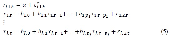
Consider a prediction regression of the form:

where
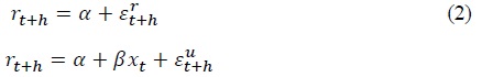
In order to exercise out-of-sample predictability test, we assume the following unrestricted and restricted prediction regression as in Equation (2). We employ the first
To compare forecast accuracy of the competing models, the out-of-sample forecast error from the unrestricted and the restricted model and the corresponding mean squared error (MSE) are calculated. The Theil’s U statistic is obtained as follows,
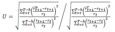
where 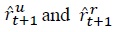 are the out-of-sample predicted value from the unrestricted and the restricted prediction model, respectively. When
Clark and McCracken (2001) estimate the forecasting model in Equation (2) and derive the ENC-NEW test statistic for forecast encompassing in Equation (3) as an alternative to comparing the forecast accuracy between the competing models:

where 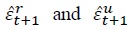 are the estimated forecast errors from the restricted and unrestricted model, respectively. If we fail to reject the null hypothesis that the restricted model encompasses the unrestricted model, then the unrestricted model is statistically insignificant in improving the predictability of cryptocurrency returns using the forecasting variable. When the competing models are nested models, as is the case in our approach, we derive the bootstrapped critical values that are immune from data mining due to the non-pivotal limiting distribution of the test statistics.
McCracken (2007) estimates the forecasting model in Equation (2) and derive the MSE-F test statistic under the null hypothesis that the MSE from the restricted prediction model is equal to the MSE from the unrestricted prediction model against the one-sided alternative hypothesis. The MSE-F statistic can be represented as follows,

where  are the estimated forecast errors from the restricted and unrestricted model, respectively. If we fail to reject the null hypothesis, then the unrestricted model is not superior in predictability to the restricted model. McCracken (2007) also shows that the MSE-F statistic is distributed to a non-standard and non-pivotal limiting distribution. As with the case of the ENC-NEW statistic, we use the data mining bootstrapped critical values to test the null hypothesis.
2. Test Procedure
It is generally the case that the returns of portfolios of financial assets are used in predictability tests of financial asset returns to reduce the dimension of the multivariate distribution of returns and the estimation errors. In the empirical analysis below, the inclusion of a certain cryptocurrency into a portfolio is confined to a few cryptocurrencies and hence dependent upon data availability. In this sense, our analysis is exposed to a risk of data mining as pointed out by Aldous (1989). In addition, the null distributions of the in-sample and out-of-sample predictability test statistics are significantly different from those of the classical test statistics. As a result, the classical in-sample and out-of-sample predictability tests on the portfolio are likely to induce size distortions.
If the critical values from data mining are employed for tests of predictability, then the null hypothesis of no predictability would be rejected too often under the given level of significance. To address the issue of size distortions due to data mining, we use a data mining robust bootstrap procedure to construct critical values for the in-sample and out-of-sample tests of predictability. We use the bootstrap procedure due to Rapach and Wohar (2006) where they develop the procedure to investigate both in-sample and out-of-sample predictability of the returns on the S&P 500 and CRSP portfolio by the nine financial fundamentals. The procedure of Rapach and Wohar (2006) can be executed by the following steps. First, we estimate the restricted prediction regression under the null hypothesis in Equation (2) and the lag
where the disturbance vector, 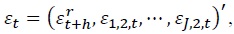 is independently and identically distributed with covariance matrix
III. Estimation
1. Data
Figure 1 shows the daily closing prices and the continuously compounded returns on the Bitcoin, Ethereum, and the Ripple Coin during the period from November 14, 2017 to June 26, 2023 (1,415 observations). As shown in Figure 1, the cryptocurrency prices have been extremely volatile during the sample period with ranging from 3.7 million KRW to 81.9 million KRW for the Bitcoin, from 97,030 KRW to 5.9 million KRW for the Ethereum, and from 182 KRW to 4,550 KRW for the Ripple Coin. The development of daily trading amount in KRW for the same period is presented in Figure 2. The daily trading amount peaked at 2.2 trillion KRW on December 8, 2017 when the Bitcoin closing price was at 20.7 million KRW. For the Ethereum, the peak was at 2.9 trillion KRW on May 13, 2021. For the Ripple Coin, the daily trading amount reached the maximum at 5.4 trillion KRW on May 19, 2021.
The three dependent variables are the log returns on the Bitcoin, Ethereum, and the Ripple Coin (BTC, ETH, and XRP). We employ two types of explanatory variables, asset-specific and non-asset-specific variables as regressors in the prediction regression of cryptocurrency returns. The explanatory variables include daily trading amount of cryptocurrency (BTC.VOL, ETH.VOL, and XRP.VOL), New York Mercantile Exchange gold futures price in USD per ounce (GOLD), US dollar index (DXY)1, implied volatility index of the KOSPI (VKOSPI), NYNEX oil futures price in USD per barrel (WTI, DUBAI, and BRENT). The daily developments of the GOLD, VKOSPI, and the DXY are shown in Figure 3, and the descriptive statistics are reported in Table 1. While the distribution of returns on the Bitcoin and the Ethereum are skewed to the left, the distribution of returns on the Ripple Coin are skewed to the right. Also, the return distributions have fatter tails than the normal distribution in all cryptocurrencies returns. The minimum daily return on the cryptocurrency is -59.41 percent in Ethereum, and the maximum daily return on the cryptocurrency is 63.59 percent in Ripple Coin. The volatility in the cryptocurrency market is the highest with the standard deviation of 7.37 percent in Ripple Coin, and the lowest with the standard deviation of 4.45 percent in Bitcoin. The Jarque-Bera test for normality is rejected at the 1 percent significance level for all variables. The daily changes in trading amount are quite volatile. The volatility in the daily trading amount is the highest with the standard deviation of 59.16 percent in Ripple Coin, and the lowest with the standard deviation of 41.74 percent in Bitcoin.
2. In-Sample Test
The extant literature on financial asset return predictability tests has used portfolio returns as dependent variables rather than individual asset returns, where the portfolios are composed based on some attributes of financial assets. Grouping cryptocurrency returns by some statistical attributes such as market capitalization in a variety of ways is difficult to exercise due to the limited number of cryptocurrency data. Also, to control for the size distortion of the predictability tests induced by grouping cryptocurrency returns based on statistical attributes derived from our own data set, we conduct in-sample and out-of-sample predictability tests of cryptocurrency returns on the individual cryptocurrency as well as on the value-weighted portfolio in this paper.
Table 2 summarizes in-sample estimation results for the Bitcoin return prediction model over the forecasting horizons up to ten days. The numbers in the table report the OLS estimates of the slope coefficient from Equation (2), and the numbers in parentheses are the p-values of the test statistics under the null hypothesis that the estimated slope coefficient is equal to zero. The critical values to test for the null hypothesis are derived from the data mining bootstrap procedure.
The coefficient estimates of the trading amount (BTC.VOL) suggest that when the daily trading amount increases the Bitcoin return increases. The exuberance in the cryptocurrency market induces potential investors to buy the cryptocurrency. The return on the Bitcoin is significantly affected by the demand for the Bitcoin. From Figure 1 and Figure 2, we can observe that the fiery increase in the cryptocurrency price and the explosive growth in the trading amount are concurrent. As the cryptocurrencies become attractive not only as a medium of exchange but as an investment opportunity, the demand for cryptocurrency has increased which would in turn increase returns on cryptocurrency investment. According to the estimation results in Table 2, the Bitcoin returns are predictable in-sample, especially for forecasting horizons from eight to ten days at the ten percent level of significance.
The coefficient estimates of the VKOSPI, though they are statistically insignificant, predict that an increase in the implied volatility of the stock market index returns results in a rise in the Bitcoin return. Since the rise in the implied volatility is indicative of the imminent upsurge in market risk, an increase in the VKOSPI would increase the demand for cryptocurrency for investors to hedge against market risk.
On the contrary to the result, the return on Bitcoin is expected to be negatively affected by the changes in the levels of WTI, GOLD, and the DXY (the dollar’s value relative to the Euro, JPY, GBP, CAD, SEK, and the CHF). Although the statistical significance of the three forecasting variables is not verified, the WTI, GOLD, DXY, and the BTC seem to have similar attributes as alternative investment opportunities. The empirical results show that Bitcoin can be viewed as an alternative hedging instrument against the traditional safe haven assets such as the US dollar or gold. Therefore, Bitcoin can be regarded as having risk management potentiality against the US dollar or gold. However, we could have expected exactly the opposite estimation results for the WTI, GOLD, and the DXY. For example, if we focus on a medium of exchange function of the cryptocurrency, the appreciation in the relative value of the US dollar would increase imports into the US. This in turn increases the demand for and the return on Bitcoin due to its currency similarity as a medium of exchange. A variety of counteractive effect on the demand for cryptocurrency would determine the direction of change in the cryptocurrency prices.
The in-sample predictability of the Ethereum returns by the ETH.VOL, BRENT, GOLD, DXY, and the VKOSPI variables over the forecasting horizons up to ten days are reported in Table 3. The coefficient estimates of the trading amount (ETH.VOL) are all positive over the forecasting horizons. Using the bootstrapped critical values, the returns on Ethereum can be significantly predictable by the ETH.VOL over the short horizons and the long horizons. As Ethereum attracts more trading amount, the price of Ethereum gets higher, or vice versa.
The coefficient estimates of the VKOSPI are all positive and statistically significant over three-to-ten-day forecasting horizons. Since the increase in the implied volatility of the stock market index returns (VKOSPI) may suggest a fear for market instability, it may stimulate investors’ interest in cryptocurrency and thereby increase the return on cryptocurrency to hedge against market risk.
The estimates of the GOLD and the DXY are negative in the Ethereum return prediction regressions, though they are not statistically significant, over the whole forecasting horizons as reported in Table 3. The GOLD, DXY, and the ETH seem to share characteristics which hedging instruments have in common. When investors take notice of imminent market risks, they increase the demand for one of these alternative assets and thereby increase the returns on the asset. As with Bitcoin, Ethereum can also be held for risk management purpose against the US dollar or gold.
The in-sample predictability of the Ripple Coin returns by the XRP.VOL, DUBAI, GOLD, DXY, and the VKOSPI variables over the forecasting horizons up to ten days are reported in Table 4. The coefficient estimates of the trading amount (XRP.VOL) are all positive over the forecasting horizons. Using the bootstrapped critical values, the returns on Ripple Coin can be significantly forecasted by the XRP.VOL over the ten-day forecasting horizons except three-to-four-day forecasting horizons. The return on Ripple Coin is the most predictable by the trading volume among other variables. Even though the sign conventions for other forecasting variables are satisfied, none of the estimates are statistically significant.
Since the increase in the implied volatility of the stock market index returns (VKOSPI) may suggest a fear for market instability, it may stimulate investors’ interest in cryptocurrency and thereby increase the return on cryptocurrency to hedge against market risk. The estimates of the DUBAI, GOLD and the DXY are negative in almost all estimates of the Ripple Coin return prediction regressions, though they are not statistically significant, over the whole forecasting horizons as reported in Table 4. The DUBAI, GOLD, DXY, and the XRP seem to share characteristics which hedging instruments have in common. When investors take notice of imminent market risks, they increase the demand for one of these alternative hedging assets and thereby increase the returns on the asset. As with Bitcoin and Ethereum, Ripple Coin can also be held for risk management purpose against the US dollar or gold.
Table 5 reports the estimation results for the value-weighted portfolio return prediction regression, where the portfolios are composed of the three cryptocurrencies, the Bitcoin, Ethereum, and the Ripple Coin. The in-sample predictability of the value-weighted portfolio returns by the WTI, GOLD, DXY, and the VKOSPI variables over the forecasting horizons up to ten days are reported. Even though the sign conventions for the forecasting variables are satisfied except for a few forecasting horizons of the WTI, none of the estimates of the forecasting variables are statistically significant.
3. Out-of-Sample Test
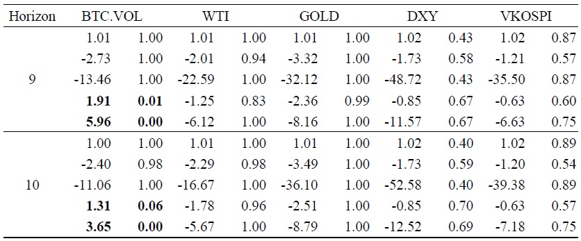
We report out-of-sample forecasting results for the Bitcoin returns over the forecasting horizons of one-to-ten days in Table 6. Each column for individual explanatory variable is divided into two columns where the first column shows the test statistics, the Theil’s U, MSE-T, MSE-F, ENC-T, and the ENC-NEW from the first row to the fifth for each forecasting horizon, and the second column presents the p-values to test for the null hypothesis of the corresponding statistic. The critical values to test for the null hypothesis are derived from the data mining robust bootstrap procedure.
The ENC-NEW test statistic for the BTC.VOL suggests that the restricted model does not encompasses the unrestricted model, then the unrestricted model is statistically significant in improving the predictability of ETH returns using the BTC.VOL variable. The out-of-sample predictability test for the BTC returns by the BTC.VOL is in line with the in-sample predictability test. However, we fail to find any evidence of out-of-sample predictability of the BTC returns by the VKOSPI variable which we find it statistically significant in forecasting the BTC returns in-sample. In addition to that, we fail to reject the null hypothesis that the MSE from the restricted prediction model is equal to the MSE from the unrestricted prediction model. That is, we have the conflicting result that the unrestricted model is not superior in out-of-sample predictability to the restricted model.
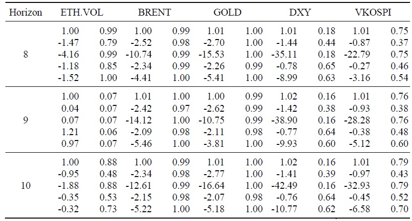
The out-of-sample forecasting results for the Ethereum returns over the forecasting horizons of one-to-ten days are presented in Table 7. From the in-sample predictability test, we find that the increase in the implied volatility of the stock market index returns (VKOSPI) stimulate investors’ interest in cryptocurrency and thereby increase the return on Ethereum to hedge against market risk. However, we do not find any evidence of the out-of-sample predictability of the return on Ethereum by the forecasting variables. The ENC-NEW test statistic of the BRENT variable for the forecasting horizon of one day is the only occasion where the restricted model fails to encompass the unrestricted model. That is, the unrestricted model is statistically significant in improving the predictability of the ETH return using the BRENT variable for the forecasting horizon of one day. Other than that, we fail to find any evidence of out-of-sample predictability of the ETH returns by the forecasting variables. In addition to that, we fail to reject the null hypothesis that the MSE from the restricted prediction model is equal to the MSE from the unrestricted prediction model. We can conclude that the unrestricted model is not superior in out-of-sample predictability to the restricted model.
The out-of-sample forecasting results for the Ripple Coin returns are shown in Table 8. From the out-of-sample predictability test results of the returns on XRP by the forecasting variable XRP.VOL presented in the first column of Table 8, the restricted model fails to encompass the unrestricted model. Therefore, the unrestricted model is statistically significant in improving the predictability of the XRP return using the XRP.VOL variable except for a few forecasting horizons. For the other forecasting variables, we fail to find any evidence of out-of-sample predictability of the XRP returns. In addition to that, we fail to reject the null hypothesis that the MSE from the restricted prediction model is equal to the MSE from the unrestricted prediction model. We can conclude that the unrestricted model with the forecasting variable XRP.VOL is superior in out-of-sample predictability to the restricted model for all forecasting horizons.
The out-of-sample predictability test results of the returns on the value-weighted portfolio by the forecasting variable GOLD presented in the second column of Table 9 show that the restricted model fails to encompass the unrestricted model. Therefore, the unrestricted model is statistically significant in improving the out-of-sample predictability of the value-weighted portfolio returns using the GOLD variable. The unrestricted model with the forecasting variable GOLD is superior in the out-of-sample predictability to the restricted model over all forecasting horizons. For the other forecasting variables, however, we fail to find any evidence of the superiority of the unrestricted model in the out-of-sample predictability to the restricted model. For the MSE-F metric, we reject the null hypothesis that the MSE from the restricted prediction model is equal to the MSE from the unrestricted prediction model with the GOLD over two-to-seven-day forecasting horizons. For the other forecasting variables with the MSE-F metric, we fail to reject the null hypothesis of equal predictability between the two competing models.
1)The US dollar index is a weighted geometric mean of the dollar’s value relative to the Euro, JPY, GBP, CAD, SEK, and the CHF.
IV. Conclusion
Cryptocurrencies are a mixture of assets that possess the potential to be a fiat currency as a medium of exchange and an alternative commodity asset for gold that investors hold to hedge against inflation and currency depreciation. From this viewpoint on cryptocurrencies, this paper aims to investigate whether the price of cryptocurrency is influenced by the value of the US dollar, the price of a variety of investment assets such gold and oil, and the VKOSPI, an implied volatility of the KOSPI index return as a measure of impending market risk. We exercise both in-sample and out-of-sample cryptocurrency return predictability tests with forecasting variables that are assumed to have these asset characteristics.
The coefficient estimates of the trading volume in the in-sample prediction regression of cryptocurrency returns are positive over the entire forecasting horizons. As the cryptocurrency attracts more trading volume, the price of cryptocurrency gets higher, or vice versa. The irrational bubble in the cryptocurrency market induces potential investors to buy the cryptocurrency. Using the bootstrapped critical values, the returns on the cryptocurrency can be significantly predictable by the trading volume over the forecasting horizons. The predictability of the cryptocurrency returns by the trading volume is generally sustained in the out-of-sample predictability. As the cryptocurrencies become attractive not only as a medium of exchange but as an investment opportunity, the demand for cryptocurrency has increased which would in turn increase returns on cryptocurrency investment. Overall, the returns on cryptocurrencies are best predicted by the trading volume of the corresponding cryptocurrency both in-sample and out-of-sample over the forecasting horizons.
Another important forecasting variable, the VKOSPI is the implied volatility of the KOSPI which measures the imminent market risk. Since the rise in the implied volatility is indicative of the impending rise in the market risk, an increase in the VKOSPI would increase the demand for cryptocurrencies for investors to hedge against the market risk. The in-sample predictability of cryptocurrency returns is most evident in the Ethereum where the test statistics are statistically significant with the data mining robust critical values. For the Bitcoin and the Ripple Coin, however, the in-sample and the out-of-sample predictability has not been proved.
Even though the sign conventions for the other forecasting variables are satisfied, none of the estimates from the in-sample prediction models are statistically significant. The estimates of the GOLD and the DXY are negative in the cryptocurrency return prediction regressions, though they are not statistically significant, over the entire forecasting horizons. The GOLD, DXY, and the cryptocurrencies seem to share characteristics which hedging instruments have in common. When investors take notice of the imminent market risks, they increase the demand for one of these alternative assets and thereby increase the returns on the asset. As with the Bitcoin, the Ethereum and Ripple Coin can be held for risk management purpose against the US dollar or gold.
We exercise the out-of-sample predictability of the returns on cryptocurrencies with the test statistics, the Theil’s U, MSE-T, MSE-F, ENC-T, and the ENC-NEW. The critical values under the null hypothesis are derived from the data mining robust bootstrap procedure.
The ENC-NEW test statistics of the trading volume in the prediction regression for the Bitcoin and the Ripple Coin suggests that the restricted model fails to encompass the unrestricted model. Therefore, the unrestricted models are statistically significant in improving the predictability of the returns on the Bitcoin and the Ripple Coin. We fail to find any evidence of in-sample predictability of the returns on the value-weighted portfolio, however, we find the evidence of the superiority of the GOLD variable in out-of-sample predictability of the returns on the value-weighted portfolio.
From the in-sample predictability test, we find that the increase in the implied volatility of the KOSPI returns may stimulate investors’ interest in and thereby increase the return on the cryptocurrencies to hedge against market risk. However, we do not find any evidence of the out-of-sample predictability of the return on the cryptocurrencies by the VKOSPI using any of the out-of-sample predictability metrics.
The most notable result in the out-of-sample predictability test is the out-of-sample predictability of the returns on the value-weighted portfolio by the forecasting variable GOLD. The empirical results show that the restricted model fails to encompass the unrestricted model. Therefore, the unrestricted model is statistically significant in improving the out-of-sample predictability of the value-weighted portfolio returns using the GOLD variable. The unrestricted model with the forecasting variable GOLD is superior in the out-of-sample predictability to the restricted model over all forecasting horizons. For the DXY and the WTI variables, we fail to find any evidence of the superiority of the unrestricted model in the out-of-sample predictability to the restricted model. From the empirical analyses in this study, we can conclude that in-sample predictability cannot guarantee out-of-sample predictability and vice versa. This may shed light on the disparate results between in-sample and out-of-sample predictability in a large body of previous literature.
Tables & Figures
Figure 1.
Daily Prices and Log Returns on Cryptocurrencies
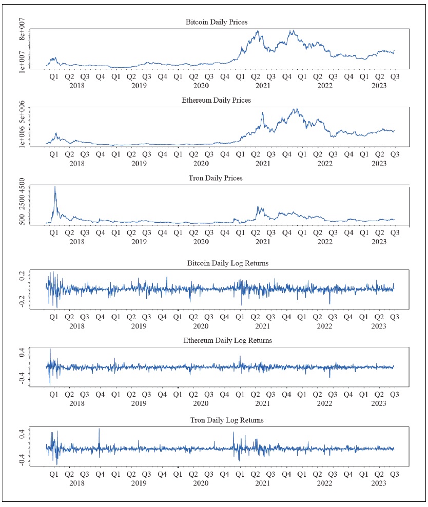
Figure 2.
Daily Trading Amount and Log Changes
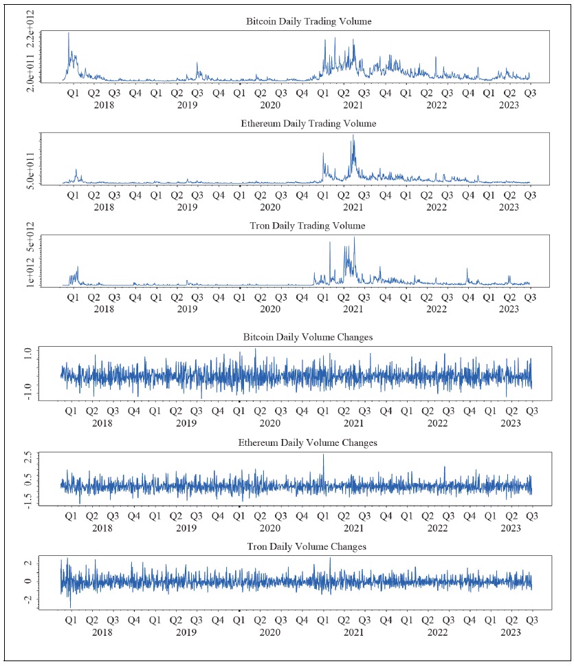
Figure 3.
Daily Development of Explanatory Variables
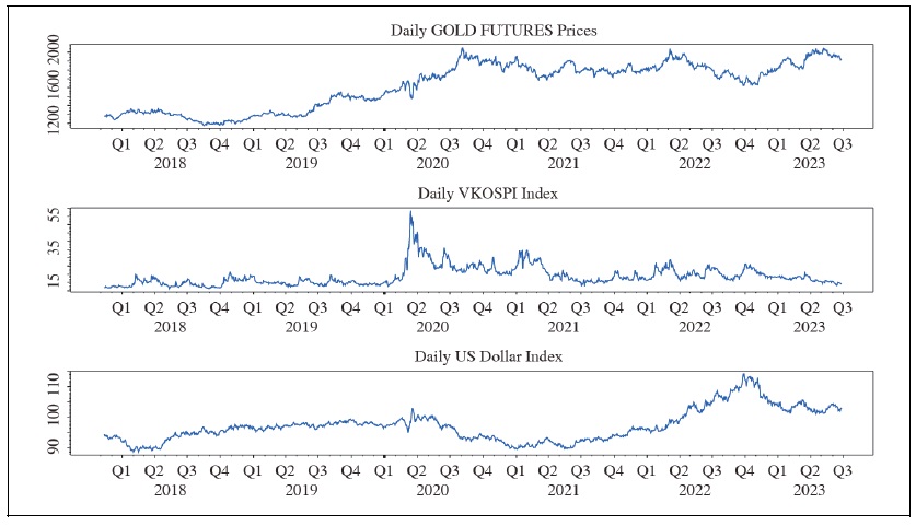
Table 1.
Statistical Summary of the Variables
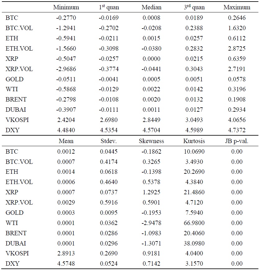
Notes: The table reports the summary statistics of the three cryptocurrencies returns and the explanatory variable used in the return prediction regression model. The numbers are reported in continuously compounded returns except VKOSPI, DXY, skewness and kurtosis. The VKOSPI and DXY are in natural logarithms. The Jarque-Bera (JB p-val.) test for normality test reports the p-values.
Table 2.
Estimation Results for the Bitcoin Return Prediction Regression
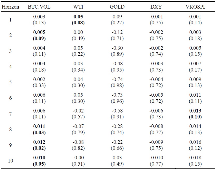
Notes: The numbers are the OLS estimates of the forecasting variables of the Bitcoin return prediction regression in Equation (2). The numbers in parentheses are the p-values to test the null hypothesis of no predictability. To derive the critical values that are immune from size distortions, we use the data mining bootstrap algorithm. The boldfaced entries denote that the estimates are statistically significant at the 10 percent level of significance.
Table 3.
Estimation Results for the Ethereum Return Prediction Regression
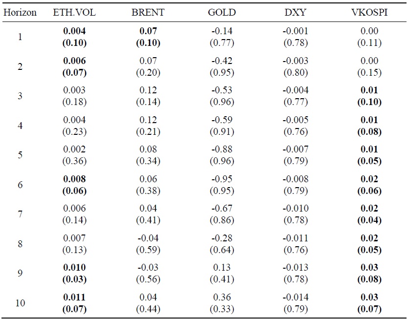
Notes: The numbers are the OLS estimates of the forecasting variables of the Ethereum return prediction regression in Equation (2). The numbers in parentheses are the p-values to test the null hypothesis of no predictability. To derive the critical values that are immune from size distortions, we use the data mining bootstrap algorithm. The boldfaced entries denote that the estimates are statistically significant at the 10 percent level of significance.
Table 4.
Estimation Results for the Ripple Coin Return Prediction Regression
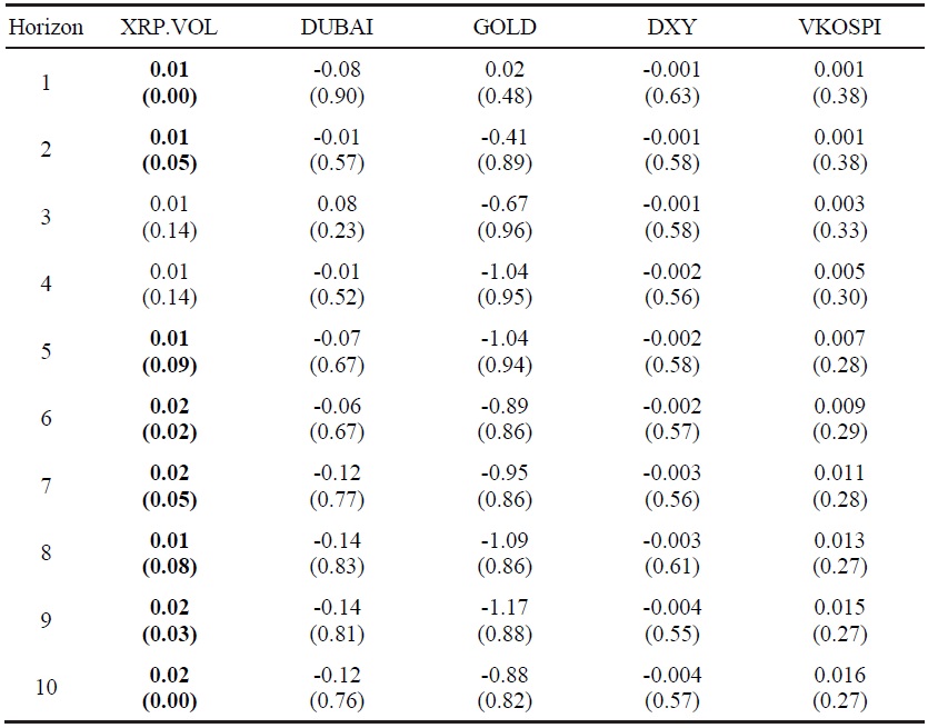
Notes: The numbers are the OLS estimates of the forecasting variables of the Ripple Coin return prediction regression in Equation (2). The numbers in parentheses are the p-values to test the null hypothesis of no predictability. To derive the critical values that are immune from size distortions, we use the data mining bootstrap algorithm. The boldfaced entries denote that the estimates are statistically significant at the 10 percent level of significance.
Table 5.
Estimation Results for the Value-weighted Portfolio Return Prediction Regression
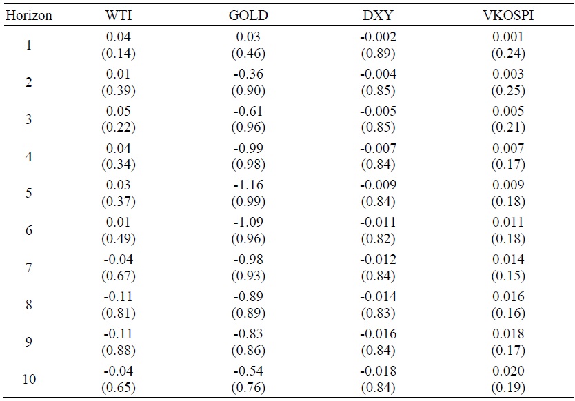
Notes: The numbers are the OLS estimates of the slope coefficient of the Bitcoin return prediction regression in Equation (2). The numbers in parentheses are the p-values to test the null hypothesis of no predictability. To derive the critical values that are immune from size distortions, we use the data mining bootstrap procedure. The numbers in boldface are used when the estimates are statistically significant at the 10 percent level of significance.
Table 6.
Out-of-Sample Predictability Test Results for the Bitcoin Return
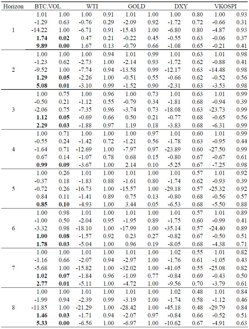
Table 6.
Continued
Notes: The out-of-sample test statistics reported in the table for each forecasting horizon are the Theil’s U, MSE-T, MSE-F, ENC-T, and the ENC-NEW statistic, respectively. Each column for individual forecasting variable is divided into two columns, where the first column presents the test statistics and the second column shows the p-values to test for the null hypothesis of the corresponding test statistic using the data mining bootstrap procedure. The numbers in boldface are used when the test statistics are significant at the 10 percent level of significance.
Table 7.
Out-of-Sample Predictability Test Results for the Ethereum Return
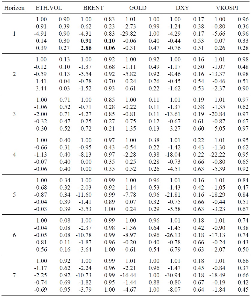
Table 7.
Continued
Notes: The out-of-sample test statistics reported in the table for each forecasting horizon are the Theil’s U, MSE-T, MSE-F, ENC-T, and the ENC-NEW statistic, respectively. Each column for individual forecasting variable is divided into two columns, where the first column presents the test statistics and the second column shows the p-values to test for the null hypothesis of the corresponding test statistic using the data mining bootstrap procedure. The numbers in boldface are used when the test statistics are significant at the 10 percent level of significance.
Table 8.
Out-of-Sample Predictability Test Results for the Ripple Coin Return
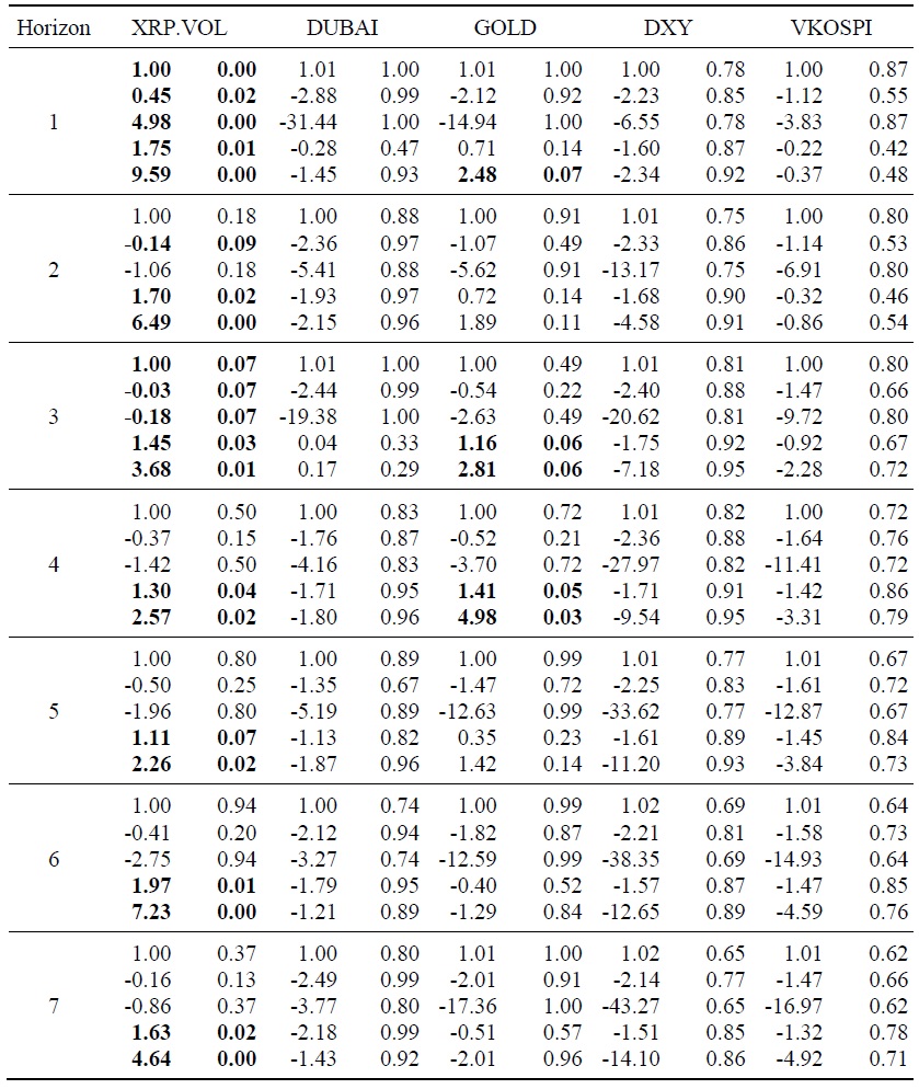
Table 8.
Continued
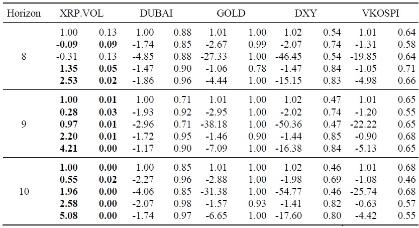
Notes: The out-of-sample test statistics reported in the table for each forecasting horizon are the Theil’s U, MSE-T, MSE-F, ENC-T, and the ENC-NEW statistic, respectively. Each column for individual forecasting variable is divided into two columns, where the first column presents the test statistics and the second column shows the p-values to test for the null hypothesis of the corresponding test statistic using the data mining bootstrap procedure. The numbers in boldface are used when the test statistics are significant at the 10 percent level of significance.
Table 9.
Out-of-Sample Predictability Test Results for the Value-weighted Portfolio Return
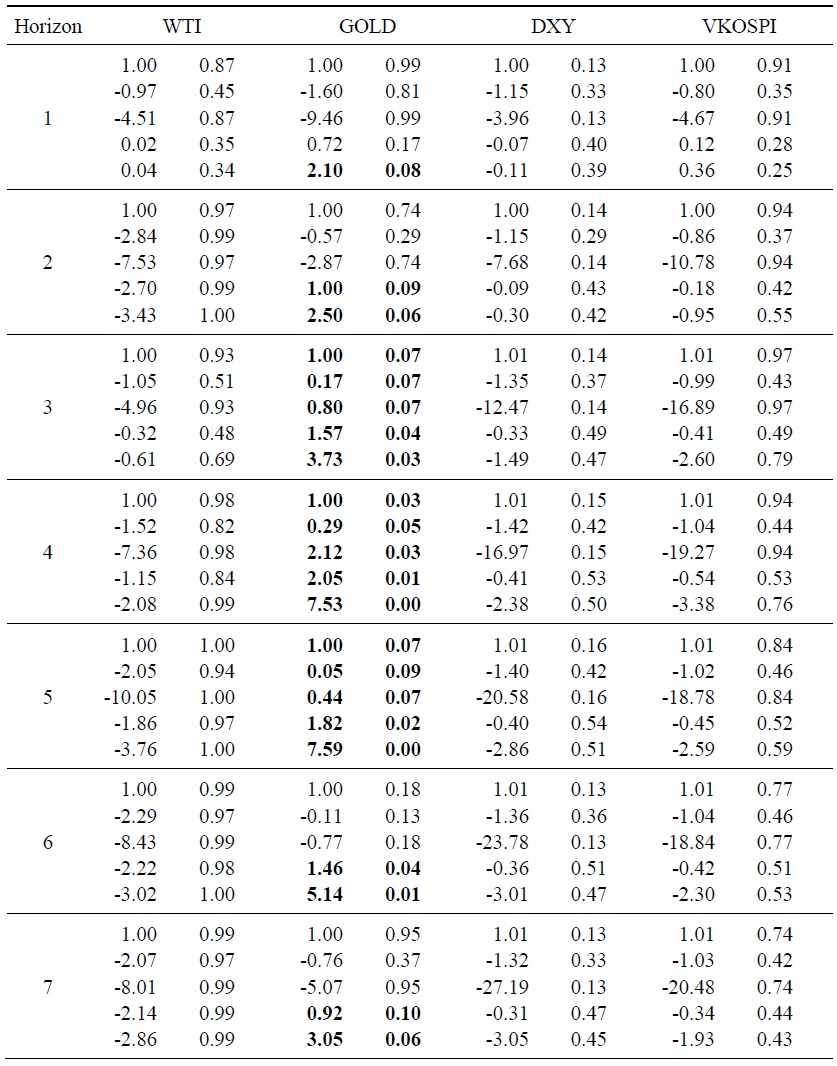
Table 9.
Continued
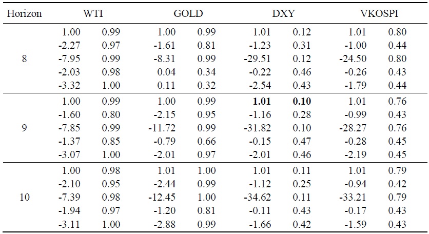
Notes: The out-of-sample test statistics reported in the table for each forecasting horizon are the Theil’s U, MSE-T, MSE-F, ENC-T, and the ENC-NEW statistic, respectively. Each column for individual forecasting variable is divided into two columns, where the first column presents the test statistics and the second column shows the p-values to test for the null hypothesis of the corresponding test statistic using the data mining bootstrap procedure. The numbers in boldface are used when the test statistics are significant at the 10 percent level of significance.
References
-
Aldous, D. 1989.
Probability Approximations via the Poisson Clumping Heuristic . Springer Science & Business Media. -
Ashley, R., Granger, C. W. J. and R. Schmalensee. 1980. “Advertising and Aggregate Consumption: An analysis of Causality.”
Econometrica , vol. 48, no. 5, pp. 1149-1167.
-
Baur, D. G., Hong, K. and A. D. Lee. 2018. “Bitcoin: Medium of Exchange or Speculative Assets?”
Journal of International Financial Markets, Institutions and Money , vol. 54, pp. 177-189.https://doi.org/10.1016/j.intfin.2017.12.004
-
Bouoiyour, J. and R. Selmi. 2015. “What Does BitCoin Look Like?”
Annals of Economics and Finance , vol. 16, no. 2, pp. 449-492. -
Buchholz, M., Delaney, J., Warren, J. and J. Parker. 2012. “Bits and Bets, Information, Price Volatility, and Demand for BitCoin.”
https://www.reed.edu/economics/parker/s12/312/finalproj/Bitcoin.pdf -
Cheah, E. T. and J. Fry. 2015. “Speculative Bubbles in Bitcoin Markets? An Empirical Investigation into the Fundamental Value of Bitcoin.”
Economics Letters , vol. 130, pp. 32-36.https://doi.org/10.1016/j.econlet.2015.02.029
-
Ciaian, P., Rajcaniova, M. and d’Artis Kancs. 2016. “The Economics of Bitcoin Price Formation.”
Applied Economics , vol. 48, no. 19. pp. 1799-1815.https://doi.org/10.1080/00036846.2015.1109038
-
Clark, T. E. and M. W. McCracken. 2001. “Tests of Equal Forecast Accuracy and Encompassing for Nested Models.”
Journal of Econometrics , vol. 105, no. 1, pp. 85-110.
-
Dyhrberg, A. H. 2016. “Bitcoin, Gold and the Dollar-A GARCH volatility analysis.”
Finance Research Letters , vol. 16, pp. 85-92.https://doi.org/10.1016/j.frl.2015.10.008
-
Foster, F. D., Smith, T. and R. E. Whaley. 1997. “Assessing Goodness-of-Fit of Asset Pricing Models: The Distribution of the Maximal R2.”
Journal of Finance , vol. 53, no. 2, pp. 591-607.https://doi.org/10.2307/2329491
-
Hanley, B. P. 2013. “The False Premises and Promises of Bitcoin.”
https://doi.org/10.48550/arXiv.1312.2048
-
Inoue, A. and L. Kilian. 2004. “In-Sample or Out-of-Sample Tests of Predictability: Which One Should We Use?”
Econometric Reviews , vol. 23, no. 4, pp. 371-402.https://doi.org/10.1081/ETC-200040785
-
Kristoufek, L. 2013. “Bitcoin Meets Google Trends and Wikipedia: Quantifying the Relationship between Phenomena of the Internet Era.”
Scientific Reports , vol. 3, pp. 1-7.https://doi.org/10.1038/srep03415
-
Kristoufek, L. and E. Scalas. 2015. “What are the Main Drivers of the Bitcoin Price? Evidence from Wavelet Coherence Analysis.”
PLoS ONE , vol. 10, no. 4.https://doi.org/10.1371/journal.pone.0123923
-
Lo, A. W. and A. C. MacKinlay. 1990. “Data-Snooping Biases in Tests of Financial Asset Pricing Models.”
Review of Financial Studies , vol. 3, no. 3, pp. 431-467.
-
McCracken, M. W. 2007. “Asymptotics for Out-of-Sample Tests of Granger Causality.”
Journal of Econometrics , vol. 140, no. 2, pp. 719-752.
-
Rapach, D. E. and M. E. Wohar. 2006. “In-Sample vs. Out-of-Sample Tests of Stock Return Predictability in the Context of Data Mining.”
Journal of Empirical Finance , vol. 13, no. 2, pp. 231-247.
-
Selgin, G. 2015. “Synthetic Commodity Money.”
Journal of Financial Stability , vol. 17, pp. 92-99.
-
van Wijk, D. 2013. “What Can Be Expected from the BitCoin?” Bachelor’s Thesis, Erasmus University.
http://hdl.handle.net/2105/14100 - Yermack, D. 2013. “Is Bitcoin a Real Currency? An Economic Appraisal.” NBER Working Papers, no. 19747. National Bureau of Economic Research.