

- EAER>
- Journal Archive>
- Contents>
- articleView
Contents
Citation
| No | Title |
|---|
Article View
East Asian Economic Review Vol. 27, No. 4, 2023. pp. 327-346.
DOI https://dx.doi.org/10.11644/KIEP.EAER.2023.27.4.427
Number of citation : 0View
35
Download
21
Business Cycle Synchronization between the European Union and Korea
|
|
Kyung Hee University |
|---|---|
|
|
The Catholic University of Korea |

Abstract
In the recent 20 years, the capital flows between Korea and European Union have increased and diversified. In particular, the business cycles of two economies have shown similar patterns since the Global Financial Crisis. This study examines both trends and investigates the roles of finance and trade on business cycle co-movements between two economies. The empirical results show that the business cycles can diverge due to either the common shocks or the country-specific shocks. Furthermore, financial integration increases the business cycle co-movements driven by both the country-specific shocks and the common shocks between two economies.
JEL Classification: E32, F40, F44
Keywords
Synchronization, Financial Integration, EU, Korea
I. Introduction
Business cycle co-movements refer to the extent to which economic fluctuations in different countries exhibit synchronicity over time. The aftermath of the Global Financial Crisis (GFC) in 2008 introduced significant shifts in global business cycles, characterized by widespread negative GDP growth rates. To counter the ensuing recession, many nations adopted historically low policy interest rates, a trend perpetuated by the subsequent European Sovereign Crisis (ESC), prolonging the period of low-interest rates and impacting the business cycles of countries globally.
Simultaneously, trade volumes and cross-border capital flows have shown a consistent uptrend since the early 2000s. China’s accession to the World Trade Organization (WTO) in 2001 played a pivotal role, amplifying global trade volumes and establishing the country as a central manufacturing hub. This transformation prompted multinational corporations to set up factories in China and other Asian countries, fostering increased international trade and interconnectedness. Consequently, global business cycles have become more aligned, influenced by factors such as trade and financial integration, coordinated monetary and fiscal policies, and other characteristics.
This study delves into the investigation of business cycle co-movements between European Union (EU) member countries and South Korea (hereafter, Korea), aiming to validate the key factors influencing this synchronization. Bilateral trades between the EU and Korea have experienced a noteworthy surge, accelerated by the signing of the Free Trade Agreement (FTA) in 2011, which dismantled trade barriers between the two regions. Over the past two decades, capital flows between Korea and EU member countries have also witnessed a significant uptick, contributing to the diversification of their economic relationships.
The distinctive feature of this research lies in its examination of financial integration and trade integration between EU and non-EU member countries, departing from the traditional focus on intra-EU nations. Additionally, we adopt a novel approach by decomposing co-movements into two types: those driven by common shocks and those driven by country-specific shocks. This methodology enables us to discern how trade and financial integration impact co-movements between a group of already synchronized countries and another country.
Empirical analysis reveals that financial integration significantly impacts business cycle co-movements to the responses of both common shocks and idiosyncratic shocks. Conditional on common shocks with heterogeneous effects, we find that financial integration has transmitted shocks to both Korea and EU member countries. In the presence of idiosyncratic shocks, both financial integration and trade integration appears to enhance economic synchronization, interpreted as amplifying the transmission of crises between the two economies.
The remainder of this paper is organized as follows. Section II presents business cycle co-movements between the EU member countries and Korea. In Section III, we discuss key variables and the empirical method. Section IV shows the empirical results, and this paper concludes with remarks in Section V.
II. Business Cycle Co-movements
1. Comparing Business Cycles
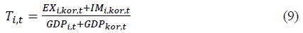
The business cycle, characterized by recurring patterns of economic expansion, contraction, and recovery, provides insights into the synchronized fluctuations of economic activities across countries. As illustrated in Figures 1 and Figure 2, GDP growth rates serve as indicators of these business cycles. Notably, the business cycles of South Korea and EU member countries undergone distinctive phases since the late 1990s.
Post the Asian currency crisis in 1998, the Korean economy rebounded sharply due to relaxed credit card issuance requirements, fostering private consumption recovery. However, this policy, aimed at boosting consumption, led to economic fluctuations in 2003, primarily confined to Korea. The mid-2000s witnessed a global economic boom before the GFC struck in 2008, impacting European economies more severely due to close financial connections with US counterparts.
Following the GFC, Korea experienced positive GDP growth, while most European countries recorded negative growth. The subsequent ESC further differentiated the economic impact, affecting the European economy more profoundly than Korea’s. In 2020, the COVID-19 pandemic prompted global economic challenges, with varying degrees of impact across countries due to differing lockdown measures.
Figure 2 depicts the GDP per capita growth rates for selected EU countries and Korea, showcasing fluctuations influenced by these events. While economic growth rates fluctuated, the responses of individual countries differed based on specific events. For instance, Germany, heavily reliant on exports, felt the impact of the mid-2000s global economic book more than other European nations. On the other hand, the ESC predominantly affected southern and emerging European countries. Despites these variations, France and Germany’s bond markets remained relatively unaffected due to their sound fiscal conditions.
2. Measuring Business Cycles Co-movements
As evidenced in Figure 1 and Figure 2, Korea and EU member countries exhibited different patterns in the early 2000s and converged post-GFC. Moreover, the comovements between Korea and each country displayed variations, influenced by country-specific or global causes. Merely comparing patterns is insufficient for a comprehensive economic explanation. To address this, previous studies have measured bilateral business cycle co-movement using negative absolute values of GDP growth rate differences (Giannone et al., 2010; Kalemli-Ozcan et al., 2013a, 2013b; Pyun and An, 2016; An et al., 2021) as in Equation (1).

where
However, Equation (1) lacks control for common shocks in GDP growth rates. Given the economic integration of EU member countries, they are inherently exposed to common shocks in GDP growth rates. This exposure is particularly pronounced in Eurozone countries, where a unified monetary policy is maintained under the control of the European Central Bank, influencing the money supply. Therefore, it becomes imperative to disentangle the effects of common shocks. Cesa-Bianchi et al. (2018) propose a methodology that decomposes  and the equilibrium response of synchronization to the common shocks,
Cesa-Bianchi et al. (2018) suggest that a true model for  a vector of common shocks
  with different country loadings,
  and the response of GDP growth rates to an idiosyncratic shock,

Then, Equation (1) can be written as in Equation (3) and are decomposed as in Equation (4) and (5):


For simplicity in presentation, the subscripts, ‘
We can conceptualize
In this study, we estimate three synchronization measures using Equation (1), (4), and (5). To estimate business cycle co-movements between EU member countries and Korea, we construct a bilateral country-panel data between 20 EU member countries (11 developed and 9 non-developed countries) and Korea.1
Initially, a straightforward principal component analysis involving 21 countries (including Korea) provides a vector of common factors based on GDP growth rates.2 Principal components are derived from the panel of 21 GDP per capita growth series in 2000-2020, with the first three principal components explaining 86.2% of total variances. Table 1 illustrates that the first principal component alone accounts for a substantial 71.7% share of total variances. The factor estimates highlight the concentration of common shocks on the first principal component, with a slightly higher value compared to Cesa-Bianchi et al. (2018) with 41 countries.
These estimated principals form a vector of fitted values of  in Equation (2). Subsequently, by conducting regressions as per Equation (6), we obtain a vector of fitted factor loadings,

Using the estimated results, we can calculate three synchronization measures. Figure 3 depicts the average of three decomposed measurements across years for 20 EU member countries. The
1)Austria, Belgium, Bulgaria*, Czechia*, Denmark, Estonia*, Finland, France, Germany, Greece*, Hungary*, Italy, Lithuania*, Netherlands, Poland*, Portugal, Romania*, Slovenia*, Sweden. * indicates that the country is classified as non-developed markets in MSCI index classification. Seven countries are excluded from 27 EU member countries: finance-focused countries (Ireland, and Luxembourg), tax-haven countries (Cyprus, and Malta), and countries with a lack of bilateral security holdings and trade data (Croatia, Latvia, and Slovakia).
2)Data section explains the selection of countries and
III. Empirical Strategy
1. Empirical Model
The conventional approach to investigating the determinates of business cycle comovements typically utilizes a bilateral country-panel regression, focusing on the characteristics of country-pairs. Noteworthy aspects in these analyses include financial integration, trade integration, industrial specialization (Imbs, 2004; Kalemli-Ozcan et al., 2013a, 2013b; Davis, 2014; Pyun and An, 2016; Cesa-Bianchi et al., 2018; An et al., 2021).
In the realm of the financial integration and business cycle co-movements, earlier studies primarily explore the benefits of financial integration on real economies (Obstfeld, 2002; Levine, 2004). However, the repercussions of financial integration on real economies have faced increased scrutiny since the Global Financial Crisis (GFC). During crises, financial linkages often serve as the primary transmission channels. Kalemli-Ozcan et al. (2013a, 2013b) demonstrate the negative effects of financial integration on business cycle synchronization, albeit limited to banking integration. Davis (2014) and Pyun and An (2016) delve into bilateral portfolio investment holdings (equity and debt), asserting that equity and debt market integration can yield distinct effects during global common shocks or the normal periods. Their analysis incorporates wealth effects and balance sheet effect explanations, emphasizing that the roles of financial integration vary based on integration types or shock origins.
Since the link between trade and business cycle co-movement established by Frankel and Rose (1998), subsequent studies have confirmed the relationship (Imbs, 2004; Di Giovanni and Levchenko, 2010; Duval et al, 2016; Cesa-Bianchi et al., 2018). However, the mechanism remains not fully understood, and empirical analysis results are mixed. Frankel and Rose (1998) propose that shocks in one country are transmitted to another country through trade, while Imbs (2004) argues that co-movements can occur even in the absence of trade. Di Giovanni and Levchenko (2010) emphasize the role of vertical production linkages, while Duval et al. (2016) explore the relationship using value-added bilateral trade data. However, Cesa-Bianchi et al. (2018) do not find a significant relationship.
This study revisits the roles of financial integration and trade integration on business cycle co-movements, differentiating between co-movements induced by common shocks and country-specific shocks. This approach facilitates a detailed examination of shock causes and their impacts. The empirical specification, resembling Kalemli-Ozcan et al. (2013a, 2013b), Cesa-Bianchi et al. (2018) and An et al. (2021), is as follows:

Here,
2. Variables
For financial market integration, we adopt a quantity-based metric commonly employed in prior studies (Kalemli-Ozcan et al., 2013a, 2013b; Davis, 2014; Pyun and An, 2016; An et al., 2021). The bilateral financial integration between country
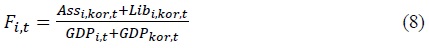
where
Similarly, trade integration (
where
To control for endogeneity among variables, additional factors such as similarities in the production structure ( where
where
As for instrument variables, the approach follows Davis (2014), Pyun and An (2016) and An et al. (2021). To identify
The initial sample period spans from 2001 when the CPIS database becomes available to 2022 for most variables. However, the Fernández et al. (2016) index is unavailable for 2020-2022, so the regression is conducted from 2001 to 2019.
Descriptive statistics for the variables employed in regressions are presented in Table 2. The table includes measures of co-movements, endogenous variables (financial integration, trade integration, and production similarity), and instrument variables. The dataset comprises 325 observations, with the stipulation that all variables must have non-missing values. In Panel B, the correlation coefficient between
IV. Empirical Results
1. The Evolution of Business Cycle Co-movements
Figure 4 shows the business cycle co-movement measures and their components by two groups of EU countries (Developed vs. Non-developed). We can find the
Figure 5 shows the evolution of financial integration (
Developed countries generally exhibit higher GDP per capita, well-established industrial bases, and sophisticated financial systems compared to less developed ones. Consequently, the vulnerability of weaker financial systems can serve as a potent channel for transmitting the impacts of global shocks to less developed countries. The increasing
2. GMM-2SLS Estimation Results
The findings from the GMM-2SLS estimation are presented in Table 3, focusing on the relationships between financial integration, trade integration, and three synchronization measures:
Moving to Table 4, which introduces additional control variables such as industrial structure similarity (I), the results mirror those in Table 3. The coefficients for financial integration remain consistent, and the p-values for Hansen’s J statistics are consistently above 10%, indicating no over-identification issues. The estimates of trade integration in columns (4)~(6) show positive signs and are significant in
Further analysis in Table 5 divides the sample period into pre-FTA (before 2011), FTA signing, and post-FTA (after 2011). Throughout the post-FTA period, financial integration remains a key factor influencing synchronization. Specifically, as depicted in Table 5, financial integration demonstrates a positive and significant impact on responses to country-specific shocks in this post-FTA timeframe. This suggests that heightened trade integration may result in interconnected capital movements between two economies, leading to synchronization not only driven by common shocks but also by idiosyncratic shocks in the business cycle. This observation aligns with findings by Cesa-Bianchi et al. (2018).
In Table 6, a comparison between developed and non-developed countries reveals variations in the impact of financial integration on synchronization. While financial integration influences both
In summary, the results consistently show that financial integration increases business cycle synchronization between EU member countries and Korea. This influence is more pronounced during the post-FTA period. Additionally, the impact of financial integration on synchronization is observed through responses to both common shocks and, post-FTA, country-specific shocks. The effects vary across country groups, with developed countries experiencing overall increased synchronization. Trade integration’s influence on synchronization varies with the inclusion of control variables, displaying results similar to prior research.
V. Conclusion
The world business cycles have shown the synchronization trend, and the European countries and Korea were no exceptions. There have been some common and country-specific shocks to economies during the last two decades. The economies responded to different degrees to the common shocks; this was also the source of desynchronization along with the difference of country-specific shocks. In particular, financial interdependence between EU member countries and Korea has deepened through increase mutual financial investments (portfolio investment holdings) after FTA signs.
Our findings highlight the impact of financial integration on business cycle synchronization. Notably, business cycle co-movements are predominantly driven by responses to idiosyncratic shocks, with the role of financial integration becoming more pronounced, particularly post-FTA signings.
Financial integration can function as either a mechanism for risk-sharing or a transmission channel for shocks between economies. In this study, we observe that financial integration between EU member countries and Korea acts as a transmission channel for the responses to both common and idiosyncratic shocks. Specifically, in the case of common shocks, financial integration transmits risks to both economies. This finding contrasts with the results of Cesa-Bianchi et al. (2018). We conjecture that EU member countries, as an economic bloc, exhibited less heterogeneous responses to common shocks. Consequently, the financial linkage in our study serves as a risk-amplifying channel rather than a risk-sharing one.
This paper contributes to the existing literature by empirically demonstrating that the roles of financial and trade integration can vary for different shocks and economic blocs. However, it is essential to acknowledge the limitations of this study. The economic definitions of common and idiosyncratic shocks are not clearly delineated. Common shocks, for instance, may encompass global events such as the GFC and the COVID-19 pandemic. However, there are distinct differences in the economic consequences between the GFC and the COVID-19 pandemic, with the former being a financial shock and the latter a medical shock. Similar distinctions apply to idiosyncratic shocks.
Future researchers can build upon our empirical methodology, extending examinations beyond the EU to encompass regions such as ASEAN countries and China. This is especially pertinent given the structural and rapid changes after COVID-19 pandemic that have implications for Korea and the broader global economic landscape.
Tables & Figures
Figure 1.
Average Growth Rates of Real GDP per Capita
Figure 2.
Growth Rates of Real GDP per Capita of Selected Countries
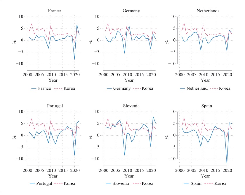
Table 1.
Factor Estimates for GDP Growth
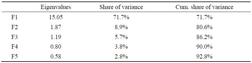
Figure 3.
The Evolution of Synchronization between EU Member Countries and Korea
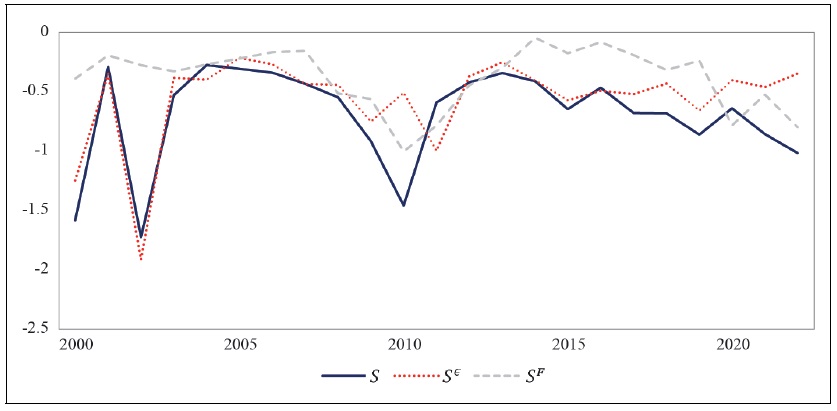
Table 2.
Descriptive Statistics of Variables
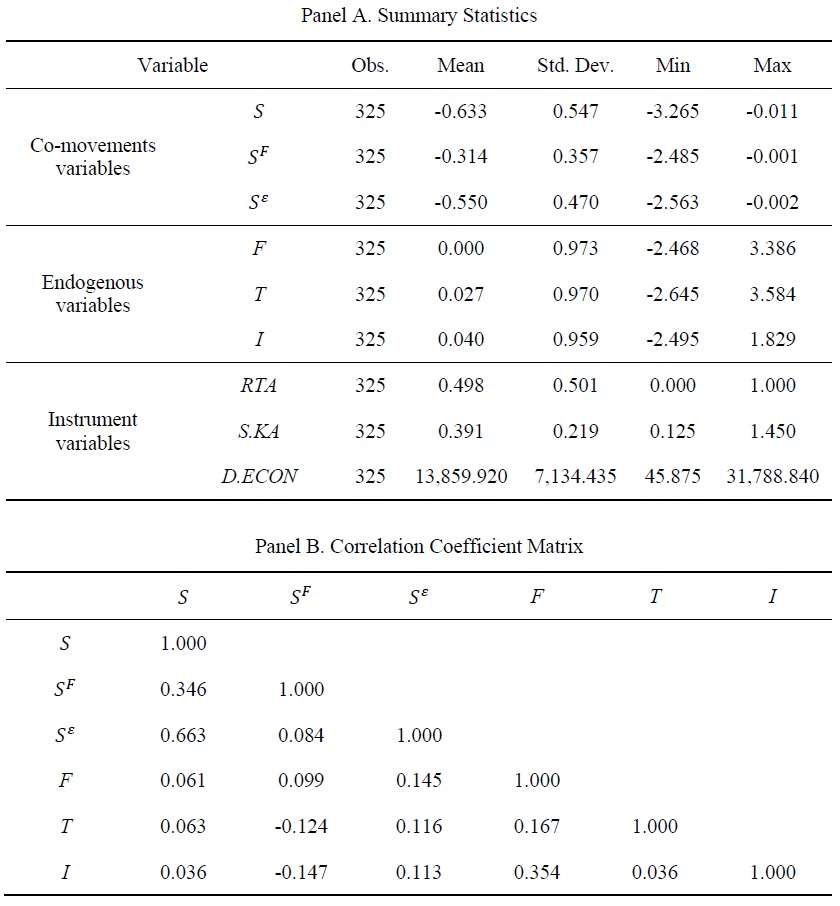
Figure 4.
The Evolution of Synchronization between EU Member Countries and Korea
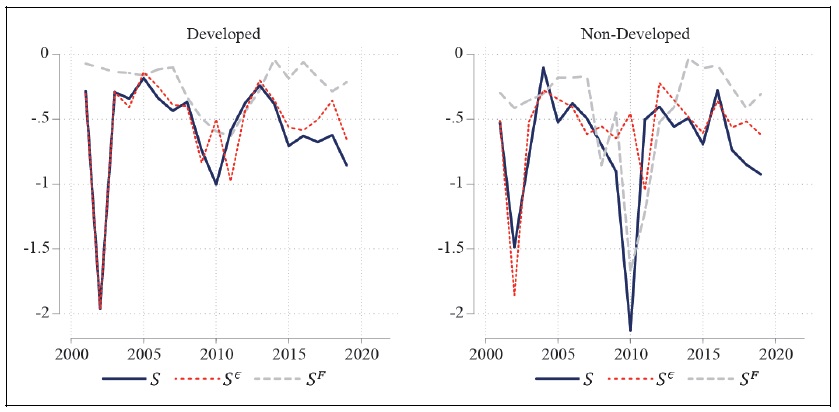
Figure 5.
The Evolution of Financial Integration, Trade Integration, and Production Similarity
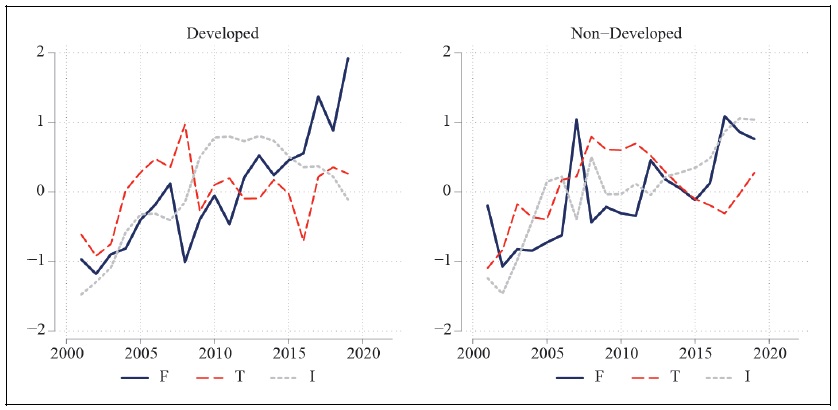
Table 3.
Synchronization, Financial Integration, and Trade Integration
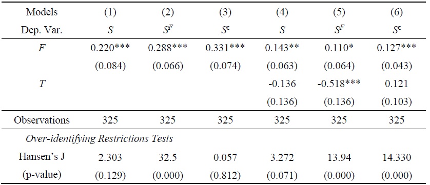
Notes: GMM-2SLS estimation is employed. Country-fixed effects are controlled. Instrumental variables are
Table 4.
Synchronization, Financial Integration, and Trade Integration with Controls
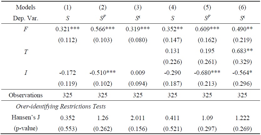
Notes: GMM-2SLS estimation is employed. Country-fixed effects are controlled. Instrumental variables are
Table 5.
The Effects of FTA
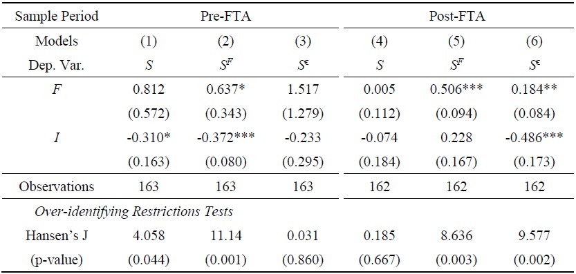
Notes: GMM-2SLS estimation is employed. Country-fixed effects are controlled. Instrumental variables are
Table 6.
Developed vs. Non-developed Countries
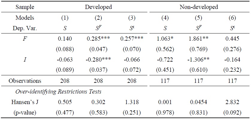
Notes: GMM-2SLS estimation is employed. Country-fixed effects are controlled. Instrumental variables are
Table A1.
List of EU Member Countries in the Analysis
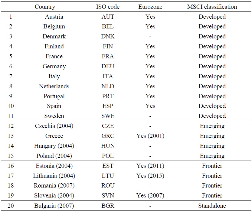
Note: Years in parentheses of the country column indicates when a country joined EU since 2000. Eurozone column also shows years in parentheses of joining Eurozone.
References
-
An, J., Kim, K. and J. H. Pyun. 2021. “Does debt market integration amplify the international transmission of business cycles during financial crises?”
Journal of International Money and Finance , vol. 115.
-
Cesa-Bianchi, A., Ferrero, A. and A. Rebucci. 2018. “International credit supply shocks.”
Journal of International Economics , vol. 112, pp. 219-237.
-
Davis, J. S. 2014. “Financial integration and international business cycle co-movement.”
Journal of Monetary Economics , vol. 64, pp. 99-111.
-
Di Giovanni, J. and A. A. Levchenko. 2010. “Putting the parts together: trade, vertical linkages, and business cycle comovement.”
Economic Journal: Macroeconomics , vol. 2, no. 2, pp. 95-124.
-
Duval, R., Li, N., Saraf, R. and Seneviratne, D. 2016. “Value-added trade and business cycle synchronization.”
Journal of International Economics , vol. 99, pp. 251-262.
-
Frankel, J. A. and A. K. Rose. 1998. “The Endogeneity of the Optimum Currency Area criteria.”
Economic Journal , vol. 108, no. 449, pp. 1009-1025.
-
Giannone, D., Lenza, M. and L. Reichlin. 2010. “Chapter 4: Business Cycles in the Euro Area.” In Alesina, A. and F. Giavazzi. (eds.)
Europe and the Euro . University of Chicago Press. pp. 141-167. -
Fernández, A., Klein, M. W., Rebucci, A., Schindler, M. and M. Uribe. 2016. “Capital control measures: A new dataset.”
IMF Economic Review , vol. 64, no. 3, pp. 548-574.
-
Imbs, J. 2004. “Trade, Finance, Specialization, and Synchronization.”
Review of Economics and Statistics , vol. 86, no. 3, pp. 723-734.
-
Kalemli-Ozcan, S., Papaioannou, E. and F. Perri. 2013a. “Global banks and crisis transmission.”
Journal of International Economics , vol. 89, no. 2, pp. 495-510.
-
Kalemli-Ozcan, S., Papaioannou, E. and J.-L. Peydro. 2013b. “Financial regulation, financial globalization, and the synchronization of economic activity.”
Journal of Finance , vol. 68, no. 3, pp. 1179-1228.
- Levine, R. 2004. “Finance and Growth: Theory and Evidence.” NBER Working Papers, no. 10766. National Bureau of Economic Research.
- Obstfeld, M. and A. M. Taylor. 2002. “Globalization and Capital Markets.” NBER Working Papers, no. 8846. National Bureau of Economic Research.
-
Pyun, J. H. and J. An. 2016. “Capital and credit market integration and real economic contagion during the global financial crisis.”
Journal of International Money and Finance , vol. 67, pp. 172-193