

- EAER>
- Journal Archive>
- Contents>
- articleView
Contents
Citation
| No | Title |
|---|
Article View
East Asian Economic Review Vol. 28, No. 1, 2024. pp. 37-67.
DOI https://dx.doi.org/10.11644/KIEP.EAER.2024.28.1.430
Number of citation : 0View
44
Download
31
The Environmental and Economic Impact of Trade between South Korea and the United States
|
|
National Korea Maritime and Ocean University |
|---|---|
|
|
Keimyung University |

Abstract
This paper analyses carbon emissions and value-added embodied in trade between two large developed countries, South Korea and the United States, during 2000-2014. Using multi-regional input-output (MRIO) tables, our analysis reveals that carbon emissions and value-added embodied in exports grew by 19% and 101% for South Korea but shrank by 43% and 7% for the United States. As a result, South Korea experienced a 40% increase in
JEL Classification: C67, F14, F18
Keywords
Decoupling Index, Carbon Intensity, Embodied Carbon Emissions, Value-added Exports, Structural Decomposition Analysis
I. Introduction
Over the past several decades, there has been an unprecedented level of globalization marked by growing international trade and investment. World trade in goods and services roughly tripled from $8 trillion to $24 trillion (2015 US dollars) between 1995 and 2021 (World Bank, 2023). This substantial growth in trade has significantly escalated its environmental impact. According to the OECD (2021), carbon (CO2) emissions embodied in trade increased by as much as 57.4% during 1995-2018. It is not surprising, therefore, that research on CO2 emissions embodied in trade has received increased attention. This line of research is crucial for understanding the drivers of CO2 emissions and designing effective mitigation policies.
A large share of research in this area has focused on CO2 emissions embodied in trade between developed and developing countries, known as north-south trade. This focus can be attributed to concerns over carbon leakage, a phenomenon resulting from the reallocation of production to countries with less stringent environmental policies. Owing to this research trend, the environmental impact of trade between developed countries, known as north-north trade, has been somewhat overlooked. Nevertheless, in 2021, the share of north-north trade at 39% outweighs that of north-south trade at 37% (UNCTAD, 2023). Moreover, the distinct characteristics of north-north trade, such as a higher prevalence of intra-industry trade, suggests that the environmental impacts are likely to differ.
This paper aims to address the existing gap in the literature by examining CO2 emissions embodied in trade between two developed countries: South Korea (hereafter referred to as Korea) and the United States (US). Bilateral trade between these two countries witnessed remarkable growth, increasing by 263% from $364B to $1,322B between 1990 and 2020, as reported by the World Integrated Trade Solutions (2023). As of 2020, the US was Korea’s second-largest export destination, while Korea was the US’ seventh-largest export destination. As of 2019, the US and Korea were the world’s second- and eighth-largest CO2 emitters. One motivation for choosing Korea and the US is that both countries have set the goal of achieving carbon neutrality by 2050. To achieve this goal, understanding the drivers of CO2 emissions resulting from international trade will be crucial.
Previous research has revealed that exports are a major source of Korea’s CO2 emissions growth (Kim et al., 2015). In fact, the share of Korea’s total emissions embodied in exports rose from 37% to 46% during 2000-2014 (Kim and Tromp, 2021). Another motivation for choosing Korea and the US is that Korea-US trade accounted for 58% of Korea’s emissions surplus and 31% of its value-added trade surplus in 2014 (Kim and Tromp, 2021). However, there have been no studies analyzing the sources of these transfers. Previous research on Korea has primarily focused on trade with China and Japan (Yu and Chen, 2017; Zhang et al., 2019; Yoon et al., 2020). Similarly, studies related to the US have primarily focused on trade with China and Japan (Zhao et al., 2016; Wang and Han, 2021; Wang and Zhou, 2019).
Another noticeable gap in the literature arises as previous research tends to focus solely on either the environmental costs or economic benefits of trade. For sustainability, however, it is necessary to analyze the environmental costs in relation to the economic benefits. The current study uses the MRIO tables from the World Input-Output Database (WIOD) to estimate CO2 emissions and value-added embodied in trade, representing environmental costs and economics benefits. MRIO tables are well-suited for this analysis because the tables capture economic and environmental linkages between industries across countries and regions. In addition, the tables enable us to mitigate the double-counting problem, which can lead to an overstatement of the economic benefits and environmental costs of trade (Liu et al., 2020; Li and Ge, 2022), by estimating value-added exports and CO2 emissions embodied in value-added exports rather than gross exports.
To compare environmental costs and economic benefits, we estimate the carbon intensity index (CI) and the decoupling index (DI). The CI shows the level of CO2 emissions per dollar of exports (Huang et al., 2019). Reductions in the CI are indicative of improvements in environmental efficiency. Two studies that estimate the CI of China’s value-added exports, rather than gross exports, are conducted by Zhao et al. (2020) and Kim and Tromp (2021). The DI, on the other hand, shows the relationship between
To reveal the primary sources of changes in CO2 emissions embodied in value-added exports, we employed structural decomposition analysis (SDA). SDA has been widely used to explore the potential drivers of changes in CO2 emissions (Su and Ang, 2012), water footprints (Feng et al., 2017), oil footprints (Wang and Jiang, 2019), energy footprints (Lan et al., 2016), and more. The SDA used in this study considers the effects of changes in production and consumption by examining the role of 10 specific factors; including emissions intensities, intermediate inputs, the final demand structure. The SDA results provide insights into the sources of changes in emissions with both domestic and international policy implications. These insights may contribute to both Korea and the US’ efforts to achieve carbon neutrality by 2050.
To summarize the main findings, CO2 emissions and value-added embodied in exports from Korea to the US grew by 19% and 101%, while those from the US to Korea shrank by 43% and 7%. Consequently, Korea’s surplus in CO2 and value-added trade with the US grew by 40% and 243%, respectively. At the industry level, the primary drivers of changes in CO2 exports were electricity and basic materials. Both countries experienced improvements in CO2 intensities, suggesting improved environmental efficiency, and a decoupling of CO2 emissions and valued-added exports, although there were year-to-year and sectoral variations. Finally, SDA reveals that domestic supply-side factors lowered emissions while foreign demand-side factors raised emissions.
1)See
2)See
II. Methodology and Data
1. The MRIO Model and Emissions Intensity of Value-added Exports
The MRIO model is widely used to measure carbon emissions and value-added flows embodied in international trade (Duarte et al., 2018; Li and Ge, 2022; Timmer et al., 2016; Wang and Han, 2021). The general formula of the basic MRIO model is

where,

where,
Let

Considering the MRIO model with


In Equation (4),
To avoid the double-counting problem in international trade, we use value-added flows. The value-added coefficients, defined as


In Equation (6),
According to the definition of the aggregate embodied intensity (AEI) (Su and Ang, 2017), we define the carbon intensity of value-added exports (CIV) for Korea and the US as
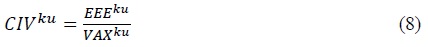
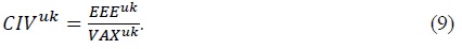

If
2. The Decoupling Model
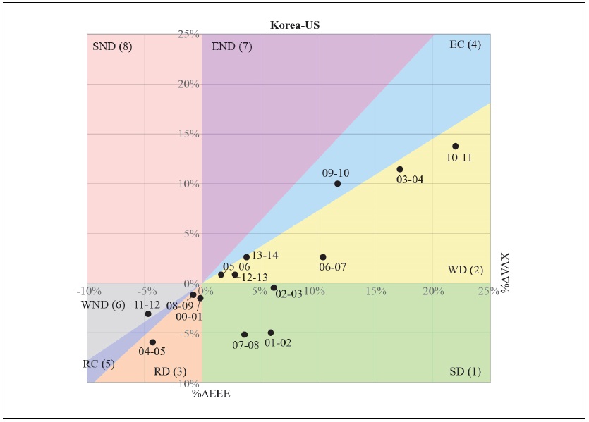
In order to analyze the decoupling states between CO2 emissions and value-added flows embodied in Korea-US trade, we use the Tapio decoupling model. The decoupling index (DI) for CO2 emissions and value-added exports in Korea-US trade between time


Here,
According to Tapio (2005), three broad states (decoupling, coupling and negative decoupling) can be further categorized into 8 detailed states based on the values and signs of the DI, Δ
3. Structural Decomposition Analysis
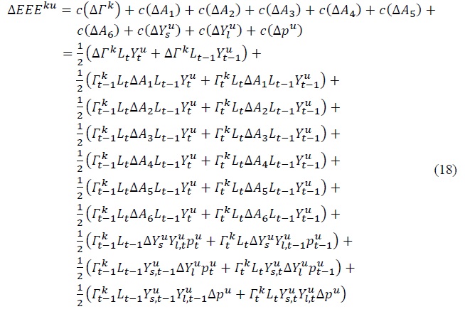
Finally, structural decomposition analysis (SDA) is used to investigate the key drivers of changes in EEE. According to Equations (4), changes in

In order to analyze more detailed factors, this study uses a two-stage SDA model that subdivides

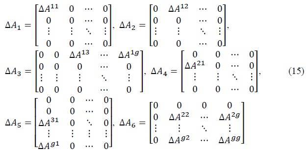
where, Δ
According to Kim and Tromp (2021), we can decompose

 obtained by dividing
  is the US’ final demand per capita and
Therefore, Δ
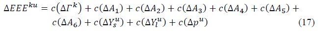
In line with Su and Ang (2012), this study uses the polar decomposition method known as the D&L method (Dietzenbacher and Los, 1998) to calculate the individual effects of the 10 factors on Δ
4. Data
This study uses the most recently published 2016 MRIO tables from the WIOD which covers 44 countries (including Korea and the US) and regions for the period 2000-2014 (Timmer et al., 2016). Each table comprises 56 sectors, and in alignment with previous studies (Wang and Yang, 2020) this research aggregates the 56 sectors into 10 industries as shown in Figure 2. This ensures more concise results and enables us to compare our findings with those in previous studies. Furthermore, we incorporate WIOD environmental accounts, which are fully consistent with the 2016 MRIO tables (Corsatea et al., 2019). The WIOD provides MRIO tables both in current prices and previous year prices, unlike other MRIO tables. In accordance with Duarte et al. (2018), we use the WIOD to construct MRIO tables in constant prices. Accordingly, our empirical analyses uncover volume effects with price effects removed.
III. Results
1. Analysis of Carbon Emissions and Value-added Exports
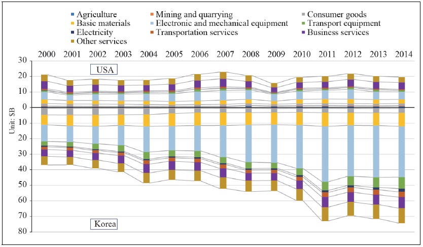
The CO2 emissions embodied in exports (EEE) and value-added embodied in exports (VAX) between Korea and the US are depicted in Figure 1. From 2000 to 2014, Korea’s VAX doubled from $37B to $74B, while its EEE increased from 41Mt to 49Mt. Until 2009, EEE fluctuated around 40Mt, despite VAX rising from $37B to $54B. The majority of Korea’s growth in EEE and VAX occurred in just two years, 2010 and 2011, with EEE rising from 39Mt to 43Mt and then to 49Mt and VAX rising from $54B to $60B and then to $73B. In contrast, the US’ VAX and EEE declined between 2000 and 2014, from $21B to $20B and 12Mt to 7Mt. The majority of the reductions in EEE occurred during 2000-2005 while VAX fell in 2001 and remained stable until 2005. There was a slight rise in EEE and VAX during 2006 and 2007, followed by a fall during the financial crisis and a subsequent recovery in 2010.
Throughout the entire study period, Korea maintained a position as a
To this end, we estimate sectoral EEE and VAX, depicted in Figure 2 and Figure 3. In the case of Korea, electricity and basic materials were the main contributors to the growth in EEE, increasing from 8.4Mt to 14.5Mt and 20.3Mt to 23.5Mt, respectively. The combined rise in EEE from these two sectors accounted for 118% of the overall growth. Conversely, consumer goods and transportation services suppressed Korea’s EEE growth, decreasing from 2.6Mt to 0.7Mt and 6.0Mt to 5.1Mt. Regarding VAX growth, electronic and mechanical equipment and transportation equipment were the main contributors, rising from $10.6B to $32.7B and $2.7B to $7.4B, constituting 72% of the overall growth. Some of this growth was offset by the decline in VAX from consumer goods from $4.2B to $2.7B. We suspect this was caused by increased competition with China since its accession into the World Trade Organization (WTO) in 2001.
For the US, EEE to Korea fell in all sectors except agriculture, which experienced only slight growth. Analogous to Korea, electricity and basic materials were the largest contributors. However, in contrast to Korea, EEE in these sectors for the US decreased from 3.7Mt to 1.4Mt and 3.7Mt to 2.5Mt, constituting 67% of the overall decline in EEE. Combined, these findings demonstrate that electricity and basic materials were key sectors driving both increases and decreases in EEE for Korea and the US. In terms of VAX, the largest contributors to the decline were other services and business services, decreasing from $4.2B to $3.5B and $4.8B to $4.4B, respectively. Once again, there was considerable concentration, with these two sectors accounting for as much as 84% of the US’ decline in VAX to Korea.
One salient trend is that sectors with large contributions to EEE tend to have small contributions to VAX, and vice versa. In 2014, basic materials and electricity accounted for 78% of Korea’s EEE but only 15% of its VAX. Similarly, for the US, these sectors accounted for 58% of EEE but only 14% of VAX. On the other hand, electronic and mechanical equipment accounted for 47% of Korea’s VAX but only 1% of its EEE, and 25% of the US’ VAX but only 4% of its EEE. The implication of these results is that valued-added exports from only a few sectors, namely basic materials and electricity, incur large environmental costs for minor economic benefits, while exports from only a few sectors, namely electronic and mechanical equipment provide large economic benefits for minor environmental costs.
The
For the US, agriculture had NE and NV surpluses with Korea during 2000-2014. Mining also had NE and NV surpluses in 2000; however, the NE surplus turned into a NE deficit during 2005-2014. In other words, the US received both economic benefits in the form of trade surpluses and environmental benefits in the form of emissions deficits from trade in mining with Korea. This suggests the use of superior environmental technologies in US mining (this is supported in the following subsection). Business services had a NV surplus and NE deficit in 2000, which also provided the US with both economic benefits and environmental benefits, but the NE deficit turned into a surplus during 2005-2014. In summary, the US received economic benefits in primary industries but environmental benefits in manufacturing and services industries from trade with Korea.
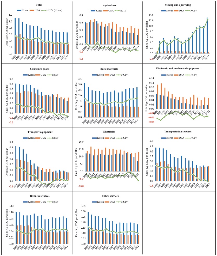
2. Analysis of the Carbon Intensity of Value-added Exports
The carbon intensity of value-added exports (CIV), representing CO2 emissions per dollar of VAX, for overall exports and sectoral exports are presented in Figure 4. The net carbon intensity of value-added exports (NCIV), from Korea’s perspective, is also included. Between 2000 and 2014, Korea’s overall CIV decreased by 41%, from 1.12kg to 0.66kg per US dollar, and the US’ overall CIV decreased by 39%, from 0.57kg to 0.35kg per US dollar. The largest reductions occurred in 2002-2004, 2007-2008 and 2011 for Korea and 2002-2006, 2009 and 2012 for the US. The substantial CIV improvements for both countries indicate a significant reduction in the environmental costs incurred to obtain the same level of economic benefits. These results suggest major improvements in environmental technologies that reduce CO2 emissions.
Korea’s CIV was substantially higher than the US’ CIV during 2000-2014, as reflected in the positive NCIV. This implies that the environmental performance of the US’ bilateral exports outmatched that of Korea. Despite this, the US was a
At the sectoral level, Korea experienced a decline in the CIV across all industries, except for mining, which exhibited an exponential increase from 0.36 to 13.06. The most significant improvement was observed in electricity, where CIV fell from 12.21 to 6.94, with the majority of the gains occurring in 2014. Transportation services also showed notable improvement, with CIV falling from 3.40 to 1.48. Although basic materials witnessed a decline in CIV from 3.15 to 2.25 during 2000-2005, it experienced a subsequent rise from 2.27 to 2.74 during 2009-2014.
In the US, CIV decreased across all industries with the most substantial improvements seen in electricity (CIV fell from 13.99 to 13.11) and basic materials (CIV fell from 1.46 to 0.97). The contributions of each sector to the overall reductions in CIV depend on their respective CIV and VAX shares. In Korea, basic materials and transportation services accounted for 51% and 21% of the reductions, respectively. The important role of transportation services is attributed to the decrease in EEE from 6.0Mt to 5.1Mt, coupled with a rise in VAX from $1.8B to $3.4B. In the US, electricity and basic materials contributed to 47% and 22% of the reductions in overall CIV.
The sectoral-level NCIV is a valuable metric for comparing the environmental friendliness of production technologies across countries. A NCIV < 0 indicates that Korea’s exports are ‘cleaner’ than those of the US, and vice versa. Comparing the sectoral-level NCIV with NE and NV allows inferences about the efficiency of the trade structure. For instance, Korea’s technological advantages in electronic and mechanical equipment and electricity (NCIV < 0), coupled with NE and NV surpluses in these sectors, can be considered environmentally efficient. In simpler terms, the US consumed ‘cleaner’ products by importing them from Korea. Conversely, the US’ technological disadvantage in agriculture (NCIV < 0), coupled with its NE and NV surpluses in these sectors, as well as the US’ technological advantages in basic materials, business services and other services (NCIV > 0), coupled with its NE and NV deficits in these sectors, can be considered environmentally inefficient. The US could potentially import ‘cleaner’ agricultural products from Korea and export ‘cleaner’ basic materials, business services and other services to Korea.
3. Decoupling Analysis of Carbon Emissions and Value-added Exports
The decoupling states, as described in Table 1, are illustrated in Figure 5 and Figure 6. As depicted in Figure 5, Korea’s exports achieved decoupling states in every period except for 2009-2010 and 2011-2012. In 12 out of the 14 periods, Korea’s exports were characterized by states of either strong decoupling (SD), weak decoupling (WD) or recessive decoupling (RD). This implies that either EEE fell despite a rise in VAX (3 periods), EEE rose at much slower rates than VAX (6 periods) or EEE fell at much faster rates than VAX (3 periods). These findings, consistent with the large reductions in carbon intensities of Korean exports, demonstrate that the economic benefits and environmental costs of trade can be decoupled despite growth in both CO2 emissions embodied in exports and growth in net CO2 emissions transfers. The two exceptions, 2009-2010 and 2011-2012, represented periods of expansive coupling (EC), when EEE and VAX rose at similar rates, and weak negative decoupling (WND), when EEE fell at slower rates than VAX. While these exceptions are challenging to explain, the return to WD in 2012-2013 and 2013-2014 suggests they may have been temporary. Overall, the prevalence of decoupling trends for exports augurs well for Korea’s road to carbon neutrality.
Figure 6 illustrates that from 2000 to 2014, the US’ exports to Korea exhibited decoupling states for 8 periods and negative decoupling states for 6 periods. Between 2001 and 2006, the US’ exports to Korea were characterized by states of SD, RD and WD. This implies that either EEE fell despite a rise in VAX (3 periods), EEE fell at a much faster rate than VAX (1 period) or EEE rose at a much slower rate than VAX (1 period). Therefore, during 2001-2006 the US consistently achieved environmentally sustainable trade with Korea. However, starting from 2006, the US’ exports were in decoupling states for only 3 of the 8 periods. For the remaining 5 periods, exports to Korea were in either END or WND states. In other words, EEE rose at much faster rates than VAX (2 periods) or EEE fell at much slower rates than VAX (3 periods). Consequently, between 2006 and 2014, negative decoupling became more prevalent for US exports to Korea. These findings are consistent with the substantial improvements in CIV until 2006 followed by stagnation until 2014.
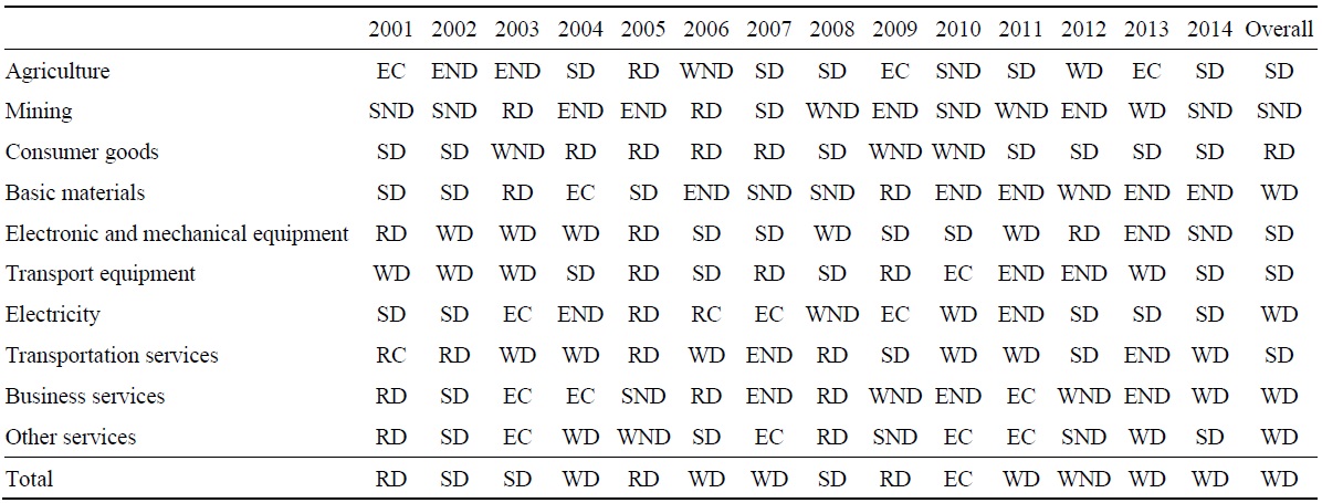
The sectoral-level decoupling states of Korea’s exports are presented in Table 3. The decoupling states were favorable in all sectors with the exception of mining. For mining, 10 of the 14 periods were characterized by states of SND (4 periods), END (4 periods) and WND (2 periods). In the case of basic materials, 8 of the 9 periods after 2005 were characterized by states of SND (2 periods), END (5 periods) and WND (1 period). Considering that mining and basic materials accounted for 61% of Korea’s total EEE growth, their unfavorable performance hindered progress in achieving environmentally sustainable trade. Agriculture, electronic and mechanical equipment, transport equipment and transportation services achieved SD overall. Although consumer goods and electricity achieved RD and WD overall, they consistently exhibited SD states during 2011-2014 and 2012-2014, respectively. Fossil fuels were the major source of power generation in Korea during 2012-2014, accounting for roughly 65% of total power generation (Statistics Korea, 2023), which rules out changes in the sources of power generation as a driver of the SD states.
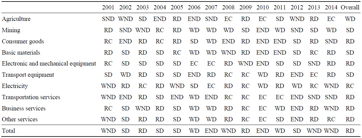
Table 4 presents the sectoral-level decoupling states of the US’ exports to Korea. During 2002-2007, the majority of industries were in decoupling states, forming the basis of the US’ environmentally sustainable exports to Korea. However, after 2007, the proportion of industries with coupling and negative decoupling states tended to increase, resulting in the US’ overall exports to Korea being in negative decoupling states for 5 out of the 8 periods. The DI of agriculture showed 5 periods of negative decoupling until 2007, but only 1 period of negative decoupling afterwards. In contrast to Korea, the US’ mining exports exhibited a strong decoupling trend, with 9 out of the 14 periods in states of decoupling. Considering the US had NV surpluses with Korea in primary industries, such improvements in decoupling indices, is positive for sustainable trade. Throughout 2000-2014, basic materials and electricity made the greatest contributions to the reduction in the US’ EEE. Basic materials had 9 periods and electricity had 7 periods of decoupling. These results suggest sustainable exports could be achieved, despite NV and NE deficits, if the US is able to continue decoupling in these key sectors.
4. Structural Decomposition Analysis of Carbon Emissions
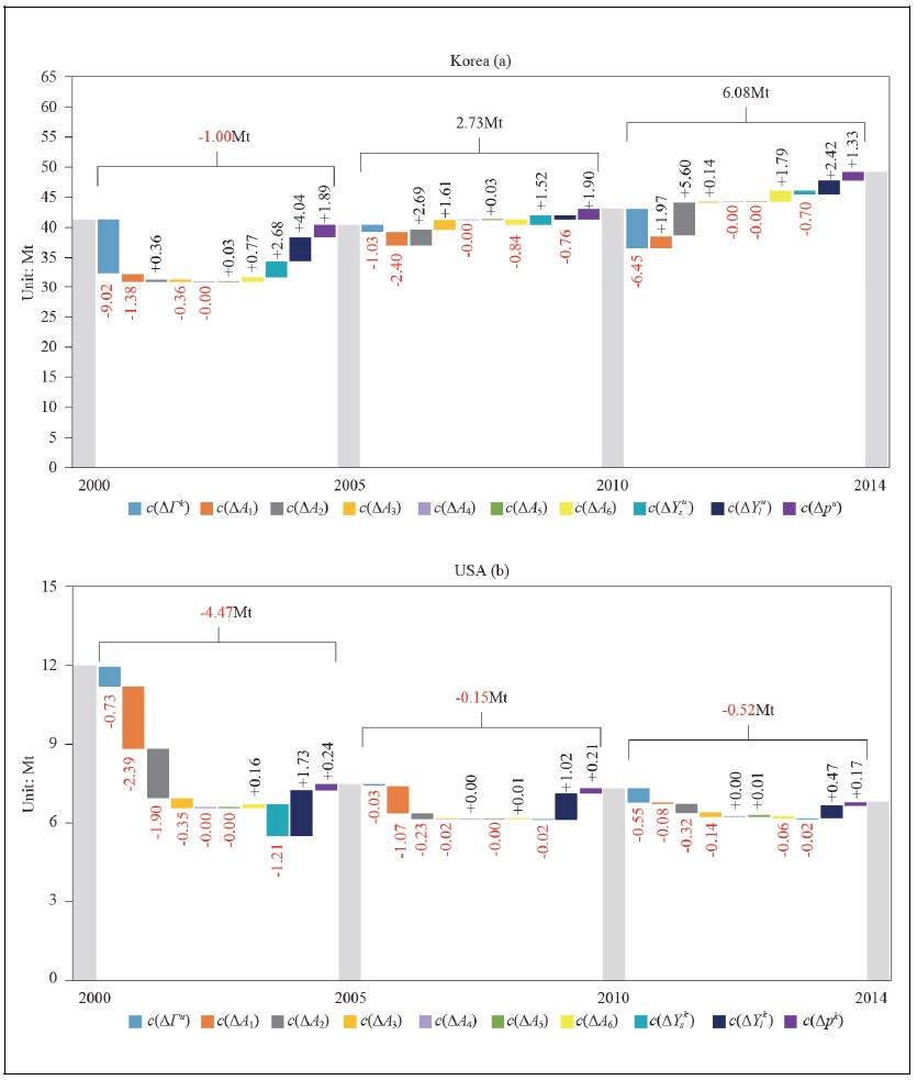
In this section, SDA is used to analyze potential drivers of the changes in EEE during the 3 distinct periods 2000-2005, 2005-2010 and 2010-2014. The estimated effects are shown in panel (a) for Korea and in panel (b) for the US.
For Korea, the most crucial factor limiting the growth of EEE appears to be changes in the CO2 emissions intensity ( Δ
Three key factors associated with the increase in Korea’s EEE were changes in the US’ final demand per capita  structure of final demand
  and population (
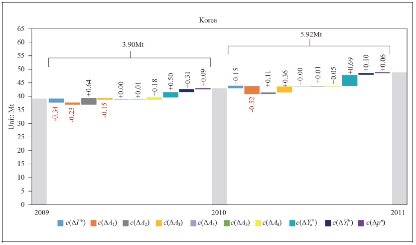
Considering that the majority of the growth in Korea’s EEE occurred in 2010 (from 39Mt to 43Mt) and 2011 (from 43Mt to 49Mt), we conduct separate SDA for Korea during these years. The figure is presented in the Appendix. In 2010, the main drivers were exports of intermediate inputs to the US (+2.48Mt), the structure of final demand in the US (+1.95Mt) and final demand per capita in the US (+1.20Mt). In 2011, the main drivers were the structure of final demand in the US (+4.10Mt) and exports of intermediate inputs to other foreign countries (+2.15Mt). This latter effect implies that Korea’s role as an upstream producer in production networks with other countries also magnified its EEE to the US. However, the fact that these effects were smaller in 2010-2014 (-0.70Mt and 0.14Mt) compared to 2010-2011 (4.10Mt and 2.15Mt) indicates that they were offset in 2011-2014.
The US’ EEE to Korea consistently decreased in the periods 2000-2005, 2005-2010 and 2010-2014. The CO2 emissions intensity (Δ
Changes in Korea’s final demand per capita  appear to have increased the US’ EEE by 1.73Mt, 1.02Mt and 0.47Mt. The positive effect for the US during 2005-2010, compared to the negative effect for Korea, are due to an increase in Korea’s final demand per capita by 14.7% during this period. Changes in the structure of Korea’s final demand
  were associated with reductions in EEE of 1.21Mt, 0.02Mt and 0.02Mt, representing a shift toward more eco-friendly consumption of final goods in Korea. Finally, population changes in Korea (Δ
To sum up, the primary factors constraining the growth of EEE growth for both Korea and the US were changes in the CO2 emissions intensity and changes in domestic intermediate inputs. Notably, these are both supply-side factors. One major difference between Korea and the US lies in the impact of their participation in international production networks as upstream producers, which tended to decrease EEE for the US but increase EEE for Korea. Conversely, the main contributors to EEE growth were final demand per capita, the structure of final demand (for Korea) and population, all of which are demand-side factors. The fact that these factors are chiefly determined abroad complicates the formulation of effective abatement policies for CO2 emissions.
3)The difference in the mean of CIV values was 0.40992 with a standard error of 0.04570 (t-value is 8.969 (p≤0.001)).
IV. Conclusions and Implications
This paper conducts a thorough analysis of changes in EEE and VAX flows between Korea and US from 2000 to 2014. The sustainability of bilateral trade is assessed using the CIV and Tapio DI. Additionally, SDA is used to analyze the driving factors behind changes in EEE. In this concluding section, we summarize the main findings and discuss their implications.
Between 2000 and 2014, both EEE and VAX increased for Korea but decreased for the US. Korea’s VAX grew more than five times faster than its EEE (101.0% vs. 18.9%) and the US’ EEE fell more than six times faster than its VAX (-43.1% vs. -6.8%). This indicates that both countries’ bilateral exports experienced decoupling states during the period 2000-2014, signaling a shift towards more environmentally sustainable trade between Korea and the US. Consistent with these findings, the CIV decreased for both Korea (from 1.12kg to 0.66kg per US dollar) and the US (from 0.57kg to 0.35kg per US dollar). In other words, the environmental costs relative to the economic benefits of trade decreased significantly over time. To achieve carbon neutrality by 2050, as both countries have pledged, without resorting to large-scale quantitative restrictions, it is crucial for these improvements in carbon intensities to persist.
Korea consistently functioned as a net carbon and net value-added exporter to the US. One interpretation of this is that Korea received net economic benefits, while the US received net environmental benefits from their bilateral trade. These imbalances, which grew substantially over time, demonstrate that carbon transfers are not exclusive to north-south but also occur in north-north trade. The implication of these transfers is that progress towards carbon neutrality may be overstated for the US and understated for Korea. However, the environmental costs of carbon transfers are not solely incurred by Korea, given their cross-border nature. Another way to interpret the net value-added and net carbon exports is that Korea benefited from production, the US benefited from consumption and the world suffered environmentally. We believe that if both countries are committed to reducing global CO2 emissions, their abatement goals must incorporate these transfers.
Both countries exhibit sectors with high EEE contributions but low VAX contributions, and vice versa. These imbalances provide valuable insights for policymakers aiming to achieve optimal abatement at the minimal costs. Industries characterized by high EEE but low VAX contributions, such as basic materials and electricity, necessitate the promotion of clean technologies or even the potential discouragement of exports. Conversely, industries characterized by low EEE but high VAX contributions, such as electronic and machinery equipment should be encouraged for exports. Both countries may find it beneficial to rationalize their tax, subsidy and tariff policies to ensure that prices better reflect the environmental costs of production, consumption, exports and imports. Alongside the development of cleaner technologies, these policy changes could contribute to rebalancing the disproportionate contributions to EEE and VAX across sectors in both Korea and the US.
One way to assess the environmental efficiency of the trade structure is by comparing NCIV, NE and NV across sectors. Our findings suggest that Korea’s NE and NV surpluses in electronic and mechanical equipment and electricity were efficient, whereas the US’ NE and NV surpluses in agriculture and NE and NV deficits in basic materials, business services and other services were inefficient. Encouraging exports from industries with NCIV advantages and discouraging those with NCIV disadvantages could be a strategic approach. If altering the trade structure proves infeasible, policymakers should focus on lowering CIV values in specific industries, given the existing trade structure. This is because a lower CIV indicates lower environmental costs (i.e., lower emissions) for the same economic benefits (i.e., valueadded exports).
The majority of Korea’s sectors tended to be in decoupling states during 2000-2014, with the exception of basic materials and mining. The US’ sectors also tended to be in decoupling states until 2007, after which many shifted to coupling or negative decoupling states. While the mining and basic materials industries experienced many years of negative decoupling in Korea, they experienced many years of decoupling in the US. These cross-country differences in sectoral decoupling provide opportunities. One option is to consider encouraging exports from sectors that are in decoupling states, which would help to reduce CO2 emissions in both countries. Additionally, gaining a better understanding of why some industries maintain decoupling states over several years while others shift between various states could provide policymakers with crucial insights into how to achieve and sustain the decoupling of CO2 emissions and exports. To the best of the authors’ knowledge, there are currently no techniques for such analyses, making this a fruitful area for future research.
The SDA revealed that domestic supply-side factors, such as CO2 emissions intensities and domestic intermediate inputs, contributed to a decrease in EEE, while foreign demand-side factors, such as final demand per capita, the structure of final demand (for Korea) and population, led to an increase in EEE. Addressing foreign demand-side factors may be challenging to undertake unilaterally. Additionally, implementing quantitative restrictions to limit the effects of final demand per capita or population may be undesirable. One potential solution is to foster cooperation to reduce EEE by promoting a cleaner structure of final demand. Korea should ensure that its high EEE exports are neither subsidized nor underpriced, while the US should work towards ensuring that its high EEE imports do not face low tariffs. Participation in international production networks as upstream producers tended to inhibit the US’ EEE but amplify Korea’s EEE. Future research should use the CIV to explore the environmental costs relative to the economic benefits of participation in these networks.
Finally, we would like to address several limitations of this research and propose suggestions for future studies. The analyses conducted throughout this work are descriptive rather than causal, revealing proximate rather than ultimate causes. With this consideration, we exercise caution in offering concrete policy implications. Nevertheless, we believe the results illuminate important patterns and raise important questions, thus establishing a solid foundation for future research. We recommend future researchers use econometric analyses to discern the ultimate causes behind many of the trends identified in this paper.
Tables & Figures
Table 1.
Decoupling States Based on the Tapio Model
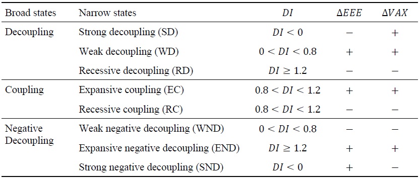
Source: Created by the author.
Figure 1.
Embodied CO2 Emissions in Exports (EEE), Value-added in Exports (VAX), Net EEE and Net VAX
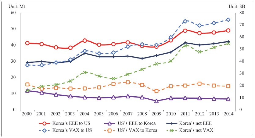
Source: Created by the author.
Figure 2.
Sectoral Structure of Embodied CO2 Emissions Exports in Korea-US Trade
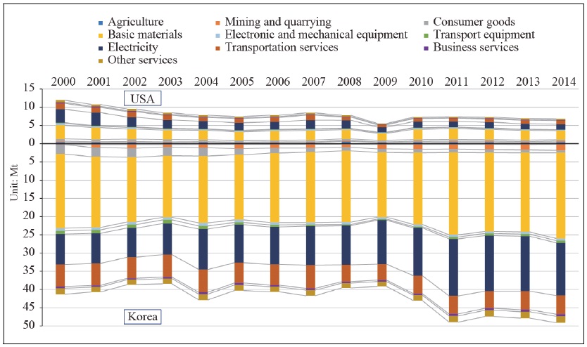
Source: Created by the author.
Figure 3.
Sectoral Structure of Value-added Exports in Korea-US Trade
Source: Created by the author.
Table 2.
Korea’s Sectoral Net EEE (NE) and Net VAX (NV) Embodied in Korea-US Trade
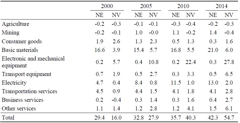
Note: NE is measured in Mt and NV is measured in billions of USD.
Source: Created by the author.
Figure 4.
The Carbon Intensity of Value-added Exports (CIV) and the Net CIV (NCIV) in Korea-US Trade
Source: Created by the author.
Figure 5.
Decoupling States between EEE and VAX in Korea-US Trade
Source: Created by the author.
Figure 6.
Decoupling States between EEE and VAX in US-Korea Trade
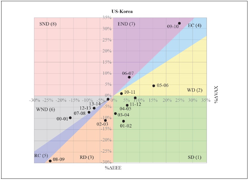
Source: Created by the author.
Table 3.
Sectoral Decoupling State in Korea’s Exports to the US
Source: Created by the author.
Table. 4.
Sectoral Decoupling State in the US’s Exports to Korea
Source: Created by the author.
Figure 7.
Contributions of Driving Factors to Changes in Korea’s EEE (a) and the US’ EEE (b)
Source: Created by the author.
Figure A1.
Contributions of Driving Factors to Changes in Korea’s EEE in 2009-2010 and 2010-2011
Source: Created by the author.
References
-
Chen, J., Wang, P., Cui, L., Huang, S. and M. Song. 2018. “Decomposition and decoupling analysis of CO2 emissions in OECD.”
Applied Energy , vol. 231, pp. 937-950.https://doi.org/10.1016/j.apenergy.2018.09.179 
- Corsatea, T. D., Lindner, S., Arto, I., Román, M. V., Rueda-Cantuche, J. M., Velázquez Afonso, A., Amores, A. F. and F. Neuwahl. 2019. “World Input-output Database Environmental Accounts (update 2000-2016).” JRC Techinical Report, no. JRC116234. European Commission, Joint Research Centre.
-
Dietzenbacher, E. and B. Los. 1998. “Structural decomposition techniques: Sense and sensitivity.”
Economic Systems Research , vol. 10, no. 4, pp. 307-324.https://doi.org/10.1080/09535319800000023
-
Duarte, R., Pinilla, V. and A. Serrano. 2018. “Factors driving embodied carbon in international trade: A multiregional input-output gravity model.”
Economic Systems Research , vol. 30, no. 4, pp. 545-566.https://doi.org/10.1080/09535314.2018.1450226
-
Feng, L., Chen, B., Hayat, T., Alsaedi, A. and B. Ahmad. 2017. “The driving force of water footprint under the rapid urbanization process: a structural decomposition analysis for Zhangye city in China.”
Journal of Cleaner Production , vol. 163, suppl. 1, pp. S322-S328.https://doi.org/10.1016/j.jclepro.2015.09.047
-
Huang, R., Lenzen, M. and A. Malik. 2019. “CO2 emissions embodied in China’s export.”
Journal of International Trade & Economic Development , vol. 28, no. 8, pp. 919-934.https://doi.org/10.1080/09638199.2019.1612460
-
Huang, Q., Xia, X., Liang, X., Liu, Y. and Y. Li. 2022. “Is China’s Equipment Manufacturing Export Carbon Emissions Decoupled from Export Growth?”
Polish Journal of Environmental Studies , vol. 31, no. 1, pp. 85-97.https://doi.org/10.15244/pjoes/139098
-
Kim, T. J. and N. Tromp. 2021. “Analysis of carbon emissions embodied in South Korea’s international trade: Production-based and consumption-based perspectives.”
Journal of Cleaner Production , vol. 320.https://doi.org/10.1016/j.jclepro.2021.128839 -
Kim, Y. G., Yoo, J. and W. Oh. 2015. “Driving forces of rapid CO2 emissions growth: A case of Korea.”
Energy Policy , vol. 82, pp. 144-155.https://doi.org/10.1016/j.enpol.2015.03.017
-
Lan, J., Malik, A., Lenzen, M., McBain, D. and K. Kanemoto. 2016. “A structural decomposition analysis of global energy footprints.”
Applied Energy , vol. 163, pp. 436-451.https://doi.org/10.1016/j.apenergy.2015.10.178
-
Li, R. and S. Ge. 2022. “Towards economic value-added growth without carbon emission embodied growth in North–North trade—An empirical analysis of US-German trade.”
Environmental Science and Pollution Research , vol. 29, pp. 43874-43890.https://doi.org/10.1007/s11356-021-17461-y
-
Liu, H., Lackner, K. and X. Fan. 2020. “Value-added involved in CO2 emissions embodied in global demand-supply chains.”
Journal of Environmental Planning and Management , vol. 64, no. 1, pp. 76-100.https://doi.org/10.1080/09640568.2020.1750352
-
Miller, R. E. and P. D. Blair. 2009.
Input-output analysis: foundations and extensions . Cambridge University Press. -
Nagengast, A. J. and R. Stehrer. 2016. “The great collapse in value added trade.”
Review of International Economics , vol. 24, no. 2, pp. 392-421.https://doi.org/10.1111/roie.12218
-
OECD. 2021. “Carbon dioxide emissions embodied in international trade [Data set].”
https://stats.oecd.org/Index.aspx?DataSetCode=IO_GHG_2021 (accessed March 30, 2023) -
Statistics Korea. 2023. “Power generation by energy source [Data set].”
https://kosis.kr/statHtml/statHtml.do?orgId=388&tblId=TX_38803_A016A&vw_cd=MT_ZTITLE&list_id=388_38803_004&seqNo=&lang_mode=ko&language=kor&obj_var_id=&itm_id=&conn_path=MT_ZTITLE (in Korean, accessed January 16, 2024) -
Su, B. and B. W. Ang. 2012. “Structural decomposition analysis applied to energy and emissions: Some methodological developments.”
Energy Economics , vol. 34, no. 1, pp. 177-188.https://doi.org/10.1016/j.eneco.2011.10.009
-
Su, B. and B. W. Ang. 2017. “Multiplicative structural decomposition analysis of aggregate embodied energy and emission intensities.”
Energy Economics , vol. 65, pp. 137-147.https://doi.org/10.1016/j.eneco.2017.05.002
-
Tan, H., Sun, A. and H. Lau. 2013. “CO2 embodiment in China-Australia trade: The drivers and implications.”
Energy Policy , vol, 61, pp. 1212-1220.https://doi.org/10.1016/j.enpol.2013.06.048
-
Tapio, P. 2005. “Towards a theory of decoupling: degrees of decoupling in the EU and the case of road traffic in Finland between 1970 and 2001.”
Transport Policy , vol. 12, no. 2, pp. 137-151.https://doi.org/10.1016/j.tranpol.2005.01.001
-
Tasbasi, A. 2021. “A threefold empirical analysis of the relationship between regional income inequality and water equity using Tapio decoupling model, WPAT equation, and the local dissimilarity index: evidence from Bulgaria.”
Environmental Science and Pollution Research , vol. 28, pp. 4352-4365.https://doi.org/10.1007/s11356-020-10828-7
-
Timmer, M. P., Los, B., Stehrer, R. and G. J. de Vries. 2016. “An anatomy of the global trade slowdown based on the WIOD 2016 release.” GGDC Research Memorandum, no. 162. Groningen Growth and Development Centre, University of Groningen.
https://www.rug.nl/ggdc/iframe/memoranda -
UNCTAD. 2023. “Trade structure by partner [Infographic].”
https://hbs.unctad.org/tradestructure-by-partner (accessed March 30, 2023) -
Wang, Q. and X. Han. 2021. “Is decoupling embodied carbon emissions from economic output in Sino-US trade possible?”
Technological Forecasting and Social Change , vol. 169.https://doi.org/10.1016/j.techfore.2021.120805 -
Wang, Q. and F. Jiang. 2019. “Drivers of United States oil footprints trajectory: A global assessment.”
Journal of Cleaner Production , vol. 240.https://doi.org/10.1016/j.jclepro.2019.118150 -
Wang, Q., Jiang, R. and R. Li. 2018. “Decoupling analysis of economic growth from water use in City: A case study of Beijing, Shanghai, and Guangzhou of China.”
Sustainable Cities and Society , vol. 41, pp. 86-94.https://doi.org/10.1016/j.scs.2018.05.010
-
Wang, Q. and X. Yang. 2020. “Imbalance of carbon embodied in South-South trade: Evidence from China-India trade.”
Science of The Total Environment , vol. 707.https://doi.org/10.1016/j.scitotenv.2019.134473 -
Wang, Q. and Y. Zhou. 2019. “Imbalance of carbon emissions embodied in the US-Japan trade: temporal change and driving factors.”
Journal of Cleaner Production , vol. 237.https://doi.org/10.1016/j.jclepro.2019.117780 -
World Bank, 2023. “World Development Indicators [Data set].”
https://databank.worldbank.org/source/world-development-indicators (accessed March 30, 2023) -
World Integrated Trade Solution (WITS). 2023. “Trade statistics by country [Data set].”
https://wits.worldbank.org/countrystats.aspx?lang=en (accessed March 30, 2023) -
Yoon, Y., Kim, Y. K. and J. Kim. 2020. “Embodied CO2 Emission Changes in Manufacturing Trade: Structural Decomposition Analysis of China, Japan, and Korea.”
Atmosphere , vol. 11, no. 6.https://doi.org/10.3390/atmos11060597
-
Yu, Y. and F. Chen. 2017. “Research on carbon emissions embodied in trade between China and South Korea.”
Atmospheric Pollution Research , vol. 8, no. 1, pp. 56-63.https://doi.org/10.1016/j.apr.2016.07.007
-
Zhang, B., Zhai, G., Sun, C. and S. Xu. 2021. Re-calculation, decomposition and responsibility sharing of embodied carbon emissions in Sino-Korea trade: a new value-added perspective.
Emerging Markets Finance and Trade , vol. 57, no. 4, pp. 1034-1049.https://doi.org/10.1080/1540496X.2019.1673161
-
Zhao, Y., Shi, Q., Li, H., Cao, Y., Qian, Z. and S. Wu. 2020. “Temporal and spatial determinants of carbon intensity in exports of electronic and optical equipment sector of China.”
Ecological Indicators , vol. 116.https://doi.org/10.1016/j.ecolind.2020.106487
-
Zhao, Y., Wang, S., Zhang, Z., Liu, Y. and A. Ahmad. 2016. “Driving factors of carbon emissions embodied in China–US trade: a structural decomposition analysis.”
Journal of Cleaner Production , vol. 131, pp. 678-689.https://doi.org/10.1016/j.jclepro.2016.04.11