

- EAER>
- Journal Archive>
- Contents>
- articleView
Contents
Citation
| No | Title |
|---|
Article View
East Asian Economic Review Vol. 28, No. 1, 2024. pp. 95-140.
DOI https://dx.doi.org/10.11644/KIEP.EAER.2024.28.1.432
Number of citation : 0View
43
Download
28
International Transmission of Macroeconomic Uncertainty in China: A Time-varying Bayesian Global SVAR Approach
|
|
Sungshin Women’s University |
|---|

Abstract
This study empirically investigates the international transmission of China’s uncertainty shocks. It estimates a time-varying parameter Bayesian global structural vector autoregressive model (TVP-BGVAR) using time series data for 33 countries to evaluate heterogeneous international linkage across countries and time. Uncertainty shocks are identified via sign restrictions. The empirical results reveal that an increase in uncertainty in China negatively affects the global economy, but those effects significantly vary over time. The effects of China’s uncertainty shocks on the global economy have been significantly altered by China’s WTO accession, the global financial crisis, and the recent US–China trade conflict. Furthermore, the effects of China’s uncertainty shocks, typically on inflation, differ significantly across countries. Moreover, Trade openness appears crucial in explaining heterogeneous GDP responses across countries, whereas the international dimension of monetary policy appears to be important in explaining heterogeneous inflation responses across countries.
JEL Classification: C32, E32, F41
Keywords
Uncertainty, International Transmission, Time-varying Parameter, Bayesian Global VAR, China
I. Introduction
What are the global economic implications of China’s increased uncertainty? This question has recently piqued the interest of economists and policymakers. China has the world’s second largest GDP and is one of the largest countries in the international trade market. After China’s WTO accession in 2001, the effects of China shocks on the global economy have become more significant. Thus, understanding the international transmission of Chinese factors to the global economy has recently become critical. Simultaneously, China faces significant economic uncertainty. For example, China’s growth rate has recently slowed, casting doubt on the country’s future sustainable growth. Furthermore, trade tensions between the United States and China, and recent debate on reshaping the global supply chain add uncertainty to China’s future growth trajectory. In this situation, it is critical to comprehend the global economic implications of China’s uncertainty.
Using a time-varying Bayesian global vector autoregressive model (TVP-BGVAR) and quarterly time series data for 33 developed and developing countries from 1995 to 2019, this paper attempts to estimate the global consequences of uncertainty in China. TVP-BGVAR includes GDP, inflation, equity price, short-term interest rate, exchange rate and uncertainty index (refer to it as “Unind” in Tables and Figures). Thus, the model is designed to investigate both macroeconomic and financial variables. In the model, I also include global oil prices, which is similar to previous GVAR literature. Global vector autoegressive (GVAR) model developed by Pesaran et al. (2004) is useful for considering global linkages. It is appropriately and efficiently designed to investigate the international consequences of shocks emanating from a country. It also considers country heterogeneity, so I use GVAR to shed light on the international consequences of China’s uncertainty. Trade weight is used to build global linkages. Furthermore, the relationship between China and the global economy has evolved over time. In particular, China’s WTO membership has had a significant impact on relations. Since joining the WTO, China has become one of the most important countries in the international trade market. The 2007?2008 global financial crisis and recent US?China trade conflicts are also potential triggers for structural breaks. Thus, those structural breaks should be considered to investigate the consequences of uncertainty in China on the global economy. To address this issue, this paper employs a time-varying framework. Uncertainty in China and other countries is measured using the world uncertainty index (WUI), which was developed by Ahir et al. (2022) based on the method of Baker et al. (2016) and Economic Intelligence Unit country reports. Uncertainty shocks are identified via reasonable sign-restrictions based on prior theoretical and empirical literature.
Several interesting findings are made. First, estimated time-varying impulse responses show that an increase in uncertainty in China negatively affects the global economy, but those effects significantly vary over time. China’s WTO accession, the global financial crisis, and the recent US–China trade conflict. Prior to China’s WTO accession, an increase in uncertainty has large domestic effects but relatively minor international effects. An increase in uncertainty in China has a significant and negative impact on China’s GDP and inflation, but it has only limited impacts on other countries. International effects become more significant after WTO membership. Moreover, global financial crisis and recent US–China trade tensions amplify the global negative effects of China’s uncertainty. Empirical findings suggest that structural breaks should be considered when studying China’s relationship with other countries.
Second, China’s increased uncertainty reduces GDP, inflation, and equity prices in other countries while raising the uncertainty index. However, the negative effects, which typically have an impact on inflation, vary significantly across countries. I use a Bayesian regression model with estimated time-varying impulse responses and measures of trade openness, financial openness, and monetary policy independence to identify potential determinants for those heterogeneous responses across countries. The final two variables, constructed by Chinn and Ito (2006) and Aizenman et al. (2010), are closely related to the international dimension of monetary policy (the trilemma hypothesis). Regression results reveal that trade openness is vital in explaining heterogeneous GDP responses across countries, but financial openness is not. Furthermore, the international dimension of monetary policy, typically the degree of monetary policy independence, appears to be important in explaining differences in inflation responses across countries. Increased trade openness is likely to amplify the negative effects of China-related uncertainty shocks. Because China is inextricably linked to the global economy via the international trade market, the trade channel is critical in explaining GDP responses. However, China is less integrated to international financial market; hence, financial openness is less important. Meanwhile, trade openness, in contrast to GDP, is less important in explaining inflation responses. For responses of inflation, monetary policy independence is important. The greater monetary policy independence, the less negative the effects of China’s uncertainty shocks on inflation. The regression results appear to be reasonable because monetary policy independence is closely related to central banks’ ability to stabilize inflation. Furthermore, heterogeneous responses of the uncertainty index across countries appear to be closely related to heterogeneous inflation responses.
This paper is related to several strands of literature. After the pioneering work by Bloom (2009), a large body of literature discusses the macroeconomic effects of uncertainty shocks. For example, Basu and Bundick (2017) and Leduc and Liu (2016), using closed economy dynamic stochastic general equilibrium models (DSGE), claimed that uncertainty shocks (an increase in uncertainty) can be interpreted as negative demand shocks. It has a negative impact on GDP, inflation, and other private activity. Moreover, Baker et al. (2016) constructed economic policy uncertainty index (EPU index) to track changes in policy uncertainty. They propose the “word count method” for constructing the EPU index. Essentially, this method counts the number of times the word “uncertainty” or related terms appear in newspapers. The more frequently those words appear in newspapers, the greater the economic uncertainty. They estimate structural VAR models using the EPU index and find that increasing the EPU index lowers GDP and employment. Several works in the literature create uncertainty indices based on their methods. In particular, Ahir et al. (2022) constructed quarterly world uncertainty index (WUI) for 143 countries from 1952, which I use as a proxy for uncertainty level in this paper. WUI is calculated by counting the percentage of country reports that contain the word “uncertain” (or a variant thereof ) in the Economic Intelligence Unit (EIU) country reports. Using panel VAR and the local projection method, they also demonstrate that an increase in WUI reduces GDP. Furthermore, some studies have attempted to quantify uncertainty in China and investigate the domestic effects of uncertainty on China. For instance, Huang and Luk (2020) created an EPU index for China using the method of Baker et al. (2016) and estimated VAR models. Their findings show that increased uncertainty reduces GDP, equity prices, and employment in China. Meanwhile, Davis et al. (2019) attempted to measure uncertainty in China using the same method as Baker et al. (2016), but they use different sources than Huang and Luk (2020). These studies concentrate on determining the level of uncertainty and investigating the domestic effects of uncertainty shocks in China. The present paper is closely related to those studies because it focuses on the macroeconomic effects of uncertainty in China. However, this paper focuses on international transmissions of uncertainty shocks, so it has a distinctive feature.
Some studies have examined the international transmission of uncertainty shocks, with a focus on the international effects of US uncertainty. For example, using random coefficient panel VAR model, Bhattarai et al. (2020) revealed that US uncertainty negatively affects emerging markets. Jones and Olson (2015) employed a VAR model to find empirical evidence of the negative effects of US uncertainty on other countries. In addition, Lakdawala et al. (2021) used a newly constructed US monetary policy uncertainty index to show how US monetary policy uncertainty affects global bond yields. China, like the US, is one of the most important countries in the global economy, but China’s global linkage is somewhat different. For example, China has a large share of the international trade market but is still less integrated into the international financial market. Thus channels of spillover effects of China uncertainty may differ from those of the United States. As a result, it is worthwhile to investigate China separately.
A few studies have focused on the international transmission of uncertainty shocks from the United States to China. For example, Huang et al. (2018) found unidirectional spillover from the United States to China using VAR model. In particular, Jiang et al. (2019) investigated spillovers of uncertainty between China and the US using timevarying VAR and finds that the main channel of uncertainty spillover between China and the US is bilateral trade, exchange rate, and investment sentiment. They employ time-varying VAR, which is similar to what I do in this paper, but I concentrate not only on bilateral relationships but also on relationships between large groups of countries. Using GVAR, Han et al. (2016) found that uncertainty in other developed economies, such as the EU and Japan, can affect China’s GDP and inflation, but they do not investigate the global effects of uncertainty in China. These studies look into international transmission of uncertainty shocks, but they focus on US uncertainty shocks or uncertainty transmission from other countries to China. In contrast to those studies, this paper focuses on the international transmission of uncertainty from China.
Furthermore, some studies found that the international effects of uncertainty shocks, which typically originate in the United States, vary across countries and regions. For example, Bhattarai et al. (2020) found that US uncertainty shocks affect emerging countries asymmetrically using random coefficients panel VAR and claims that different monetary policy responses to US uncertainty shocks across countries cause those heterogeneous outcomes. Carrière-Swallow and Cespedes (2013) used a VAR model to estimate the effects of global uncertainty on individual countries and discover that emerging economies suffer far more severe drops in investment and private consumption than the US and other advanced countries. Global VAR frameworks, which I use in this paper, efficiently account for those potentially heterogeneous consequences across countries.
A small body of literature focuses on the international transmission of uncertainty shocks that do not originate in the United States. For example, Belke and Osowski (2019) estimated a large-scale factor augmented VAR model using OECD countries and find that uncertainty in the US and EU reduces GDP, CPI, equity prices, and interest rates in other countries and regions. They do not, however, take China into account. Klößner and Sekkel (2014) estimated spillover effects for six developed countries (G7 countries excluding Japan) and discovers significant spillover effects among those countries.
Zhang et al. (2019) used rolling window VAR and the generalised version of the forecasting error variance decomposition (GFEVD) developed by Diebold and Yılmaz (2014) to estimate the global impacts of China’s and the United States’ EPU indexes. They come to the conclusion that China’s uncertainty has an impact on the global stock, energy, commodity, and credit markets. Their research provides some empirical evidence on the international transmission of uncertainty in China, but it is limited to a few markets. The work of Fontaine et al. (2018), which is the most relevant to this paper, used a smooth-transition VAR (STVAR) model to investigate the effects of uncertainty in China on some selected economies. They use STVAR to estimate the bilateral relationship between China and each of six economies (the United States, the Eurozone, Japan and Korea, Brazil, and Russia) and find significant spillover effects. These spillover effects are much stronger in recessions, indicating nonlinear international transmission of uncertainty in China. Their paper contributes to a better understanding of the nonlinear international transmission of China uncertainty. However, they only consider bilateral relations, so global linkage is only partially considered. For example, increased uncertainty in China may reduce output in the United States and Canada due to direct links between China and those countries. Because of the link between the US and Canada, a drop in US output can also have an impact on Canada. Bilateral relationships are incapable of properly capturing the second channel. This paper employs a global VAR model that includes 33 developed and developing countries and is capable of accurately capturing all global linkages. Furthermore, there are several potential structural breaks between China and the global economy. For example, China’s WTO accession in 2001 and the global financial crisis have the potential to alter China’s relationship with the global economy. Kim (2020) used a time-varying VAR model to provide empirical evidence on those structural breaks. Although possible nonlinearity is considered in Fontaine et al. (2018), they only considered one specific regime (recessions in a recipient country). I use a timevarying framework to better capture the effects of unknown and multiple structural breaks.
The remainder of this paper proceeds as follows. Section II presents the econometric method, identification strategy, and data. Section III provides the empirical results and relevant discussions on the results. Section IV concludes.
1)See EPU index website:
2)See
II. Econometric Method and Data
In this section, I go over specific econometric methods, data, and identification. I begin by introducing TVP-BGVAR. Then I go over identification strategies using sign restrictions. Finally, I explain the data that I use to estimate.
1. TVP-BGVAR
The TVP-BGVAR model is based on the GVAR model of Pesaran et al. (2004). The GVAR model is intended to estimate international linkages between countries using standard VAR models. GVAR is widely used in international economics literature. Although the GVAR model is designed with a linear assumption, some studies add nonlinearity to GVAR. For example, Chudik et al. (2021) extended GVAR to threshold-augmented GVAR (TGVAR) to account for regime-specific effects. Crespo-Cuaresma et al. (2019) extended GVAR to time-varying Bayesian GVAR (TVP-BGVAR) to capture unknown and multiple structural breaks of US monetary policy shocks. Unlike standard GVAR, which assumes time-invariant parameters, TVP-BGVAR allows parameters to change over time, making it useful for capturing the effects of unknown and multiple structural breaks. Böck et al. (2021) investigated the international effects of forward guidance in the Eurozone using TVP-BGVAR. I use TVP-BGVAR to account for structural breaks in China’s relationship with the global economy. Two distinct stages are used to estimate the model. First,
For the country-specific models, let endogenous variables  weakly exogenous variables
  are included in each country-specific model and are constructed with the following equation:

 is weighted average of the other countries’ endogenous variables. In equation (1),
  with
with
Endogenous variables (domestic variables) include the following six variables: GDP, CPI inflation, short-term interest rate, equity price, exchange rate vis-a-vis US dollar, and WUI. Weakly exogenous variables (foreign variables) are a collection of those variables that have been weighted averaged. For the United States, the exchange rate is not included as an endogenous variable, but the oil price is, as is customary in GVAR models. As a result, foreign variables for other countries include the price of oil. Section 2.3 contains detailed descriptions of variables and data.
Using those endogenous and exogenous variables, we can define a country-specific model as follows:

 matrix of coefficients for weakly exogenous variables. It is also allowed to vary over time. Finally,
  Here,
Here,  is a lower triangular matrix. Thus,
  where
where

where  This autoregressive log-volatility process is widely adopted in time-varying VAR model. For example, Primiceri (2005) and Cogley and Sargent (2005) also used simialr process for modelling heteroskedastic volatility in time-varying VAR model. Additionally, Stock (2001) mentioned that the time variation in VAR coefficients can be exaggerated without heteroskedastic innovations.
Then, the global model is constructed using the following step. To defined the global model, let  -dimensional vector. Using

where  country specific weighting matrix

Stacking the equations

where  and
and  The error term
  is normally distributed with mean zero and block-diagonal covariance matrix
Now, I explain how specifically parameters evolve over time. Let  be a
be a  and
and  collects all regression coefficients. Using

where 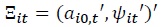 be the collecting vector where

where  is a white noise process with time-varying variance
  is assumed to be the following process following Crespo-Cuaresma et al. (2019):

 is assumed close to 0. According to Crespo-Cuaresma et al. (2019), this mixture innovation model helps mitigating the overfitting issue. Note that
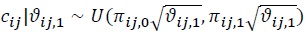
where  is
is  denote draws of the coefficients and a (latent) threshold
To estimate this model, I use the Bayesian shrinkage method described in Crespo-Cuaresma et al. (2019). Appendix A and Appendix B contain detailed markov chain monte carlo algorithms and priors for estimation. I repeat the algorithm 40,000 times and burn-in the first 30,000 draws. I keep every tenth draw of the remaining 10,000 as a posterior draw. The inferences are based on the 1,000 draws.
2. Identification
I use the structural generalized impulse response function (SGIRF) in this paper to shed light on the dynamic international effects of uncertainty in China. SGIRF is a common choice in the GVAR literature because identifying all
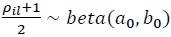
I make the following assumptions when identifying uncertainty shocks in China via sign restrictions. First, I assume that increased uncertainty in China reduces GDP and inflation. This is consistent with one popular interpretation of uncertainty shocks as negative demand shocks. Basu and Bundick (2017) and Leduc and Liu (2016) used the DSGE model to investigate the effects of uncertainty shocks and conclude that uncertainty shocks can be interpreted as negative demand shocks. This means that an increase in uncertainty negatively affects GDP and inflation. That interpretation is followed in this paper. Second, I assume that increased uncertainty in China will have a negative impact on equity prices. This is supported by empirical findings in Huang and Luk (2020) and You et al. (2017). Their findings show that an increase in uncertainty has a negative impact on equity prices in China, at least in the short run. Based on the findings, I assume that uncertainty shocks lower equity prices. Third, I do not impose any restrictions on short-term rate and exchange rate responses in China.
These two variables are closely related to China’s monetary policy. However, evidence on monetary policy responses to macroeconomic conditions in China is somewhat mixed in terms of tools and monetary policy operation. For example, Fernald et al. (2014) asserted that short-term interest rates and reserve requirements are monetary policy tools in China, whereas Chen et al. (2018) asserted that M2 is a monetary policy tool. Geiger (2008) show that China uses multiple instruments. This means that it is difficult to pinpoint China’s short-term interest rate and exchange rate responses to uncertainty shocks. Furthermore, Huang and Luk (2020) demonstrated that deposit rate responses to uncertainty shocks are not robust. Thus, I do not impose any restrictions on the responses of those variables. Finally, shocks of uncertainty raise WUI. All restrictions are only imposed in a quarter. As a result, the set of constraints can be interpreted as a minimal set of constraints. The restrictions are summarized in Table 1. Note that I introduce another shock, such as business cycle shocks that increase GDP and inflation simultaneously (no other constraints) or monetary policy shocks that increase short-term rates but decrease GDP and inflation simultaneously (no other constraints), and estimate the model with uncertainty shocks. The results, however, are not significantly different from the baseline model with the single uncertainty shock. As a result, I decide to leave out the shocks. The shock can be estimated using the following procedure using this set of constraints, the Chinaspecific model, and the algorithm of Rubio-Ramirez et al. (2010).
Let the index for the China-specific model be
By the algorithm of Rubio-Ramirez et al. (2010), rotation matrices
This
Sign restrictions are used in some studies to identify uncertainty shocks. For example, Redl (2017) and Redl (2020) used sign restrictions to investigate the macroeconomic effects of uncertainty shocks. One advantage of the sign restriction method is allowing contemporaneous interactions among variables in the system. In the literature, a short-run zero restriction via Cholesky decomposition is a popular method for identifying uncertainty shocks with VAR models. For example, Baker et al. (2016), Leduc and Liu (2016), and Bhattarai et al. (2020) used this approach to identify uncertainty shocks, though they all use different proxies of uncertainty and ordering strategies. This is a convenient and widely used method for identifying uncertainty shocks in VAR frameworks, but it is debatable. As Ludvigson et al. (2021) pointed out, this recursive structure does not allow or limit endogenous responses of uncertainty to business cycle conditions. They argue that this restriction is not only atheoretical but also a source of bias because it limits the comovements of uncertainty and business cycles, particularly during recessions. This criticism can be avoided by using the sign restriction method, which allows for simultaneous interactions among variables and can use results from theoretical models.
3. Data
The data set includes quarterly time series data for 33 countries, including both developed and developing nations. The majority of the macroeconomic data for those countries is derived from the GVAR database, which was created by Mohaddes and Raissi (2020). According to Mohaddes and Raissi (2020), these 33 countries account for roughly 90% of global GDP. They gather information from a variety of sources, including the IMF’s IFS database, Haver Analytics, and MSCI. Their data also include quarterly oil prices. The benefit of this dataset is that it is built using a consistent standard for each country. Also data set is readily available for GVAR models. TVP-BGVAR is estimated using samples from 1995 to 2019, which include several potential structural breaks such as China’s WTO membership, the global financial crisis, and the recent US–China trade war.
For most countries, I estimate using six variables: GDP, inflation, real equity index, exchange rate, short-term interest rate, and uncertainty index. GDP is defined as the log of real GDP, and the inflation rate (INFL) is defined as the log change in CPI inflation. The exchange rate (EXC) is the bilateral exchange rate (deflated using the CPI index) in relation to the US dollar. The nominal interest rate is the short-term interest rate. Equity price (Equity) is a real equity index defined as the log level of the equity index deflated using the CPI index. However, some countries’ equity indexes are missing from the data in Mohaddes and Raissi (2020). As a result, I obtained equity indexes for those countries from the CEIC database. In particular, I use the Shanghai stock exchange composite index as a proxy for China’s equity index. I use the method of Mohaddes and Raissi (2020) to convert those equity indexes to log-real variables. I include log of oil price for the United States. All variables are detrended using a linear-quadratic trend.
I use the world uncertainty index (WUI) developed by Ahir et al. (2022) as a proxy for macroeconomic uncertainty in China and other countries. WUI has the advantage of being based on a consistent method across countries, so the index is directly comparable across countries. It also covers 143 countries since the first quarter of 1952. The Economic Policy Uncertainty Index (EPU index), which can be used as an alternative uncertainty index, only covers a few countries. For example, the EPU index excludes Saudi Arabia and South Africa. As a result, I have chosen WUI as a proxy for uncertainty. Because the model includes WUI for all countries, the weighted uncertainty index is included as a weakly exogenous variable in China’s country model. The weighted uncertainty index can be interpreted as a global uncertainty excluding China, so including it aids in isolating China’s uncertainty shocks that are unrelated to global uncertainty. Figure 1 depicts the WUI for China. Large spikes have been observed around major economic events such as the Asian financial crisis in 1998, China’s WTO accession in 2001, the global financial crisis, and the Eurozone debt crisis in 2010. Finally, recent trade tensions between the United States and China have increased uncertainty in China, causing the index to reach its historical high around 2018.
Table 2 displays a list of countries as well as a classification of regions and income levels. The definition of regions is consistent with Mohaddes and Raissi (2020). As shown in the table, all major countries are included so that the model can capture the global economy efficiently. I also include the income level of the sample countries. According to the World Bank classification, high-income countries are classified as high income, while upper-middle and lower-middle income countries are classified as middle income. Among 32 recipient countries (all countries excluding China), 21 countries are in the high-income group and 11 countries are in the middle-income group.
3)
4)Some variables are not available for some countries. For example, equity price and exchange rate are not available for Saudi Arabia.
5)It is also the same with
6)Results are available upon a request.
7)More detailed discussion, particularly on issues in time-varying frameworks, is provided in
8)For Mexico, I use BMV index. For Brazil, I use Sao Paulo Stock Exchange index.
9)According to
III. Results and Discussion
In this section, I present estimated results and discuss them. First, I show some subsample VAR results that provide preliminary evidence of a structural break. Second, the TVP-BGVAR results are displayed. I try to show TVP-BGVAR results from various perspectives. I begin by displaying results for selected individual countries. Then I go over some aspects of country-level heterogeneous responses.
1. Preliminary Results: Sub-sample Time-invariant BGVAR
I show estimated impulse responses from sub-sample time-invariant Bayesian GVAR models before discussing full time-varying results. The findings suggest that there is a structural break. I divide the entire sample (1995 to 2019) into two subperiods: before the global financial crisis (from 1995 to 2008) and after the global financial crisis (from 2009 to 2019). Note that other potential break points are not feasible in this sub-sample analysis. For example, because China joined the WTO in 2001, the first sub-period is too short to estimate the model. Similarly, the recent US–China trade wars began around 2016, making the second sub-period too short. The magnitude of shocks is normalized by a unit increase in the uncertainty index, allowing results from two different sub-periods to be directly comparable. I present the results for the United States (international effects) and China (domestic effects) as preliminary evidence of a structural break. These two countries are inextricably linked by the international trade market. As a result, the findings are useful for comprehending international effects. Figure 2 depicts the results. The left panel shows the results for China, while the right panel shows the results for the United States. The blue line and shaded areas represent the median responses in the pre-financial crisis period, as well as the associated 68 percent confidence bands. The red and black dotted lines represent the median responses in the post-financial crisis period, as well as the associated 68% confidence bands. The X-axis represents a quarter after the shocks have occurred.
GDP responses in China differ significantly between two sub-periods. The GDP response on impact is large, but the negative effects are short-lived in the pre-financial crisis, whereas the response is relatively small, but the negative effects are long-lived in the post-financial crisis. An increase in uncertainty in China has a negative impact on equity prices, but the persistence differs between two sub-periods. Equity price responses in the pre-financial crisis are long-lasting, whereas those in the financial crisis are short-lived and quickly turn positive. WUI dynamics are not different across sub-periods, so differences in impulse responses across periods are unlikely to be caused by different WUI dynamics.
In terms of the shape of impulse responses, GDP responses in the United States differ slightly across time. The peak response occurs on impact in the pre-financial crisis, while it occurs after a quarter in the post-financial crisis. GDP, inflation, and equity prices all fall as a result of China uncertainty shocks, though the statistical significance is unclear. TVP-BGVAR improves statistical significance, as shown in the following subsection. It is possible that this is due to the fact that TVP-BGVAR accounts for the effects of structural breaks better than the sub-sample VAR. Nonetheless, the findings provide evidence on the international consequences of China uncertainty shocks. Finally, WUI responses in the US show relatively large spikes in the post-financial crisis period when compared to the pre-financial crisis period.
The time-invariant sub-sample VAR results show some evidence of a structural break, but not enough to provide an overall picture of China uncertainty shocks’ international transmission. This is due in part to the difficulty of considering other potential structural breaks in sub-sample VAR analysis. TVP-BGVAR results are shown in the following subsection to provide more concrete evidence on international transmission of uncertainty in China.
2. Unveiling Full-time Variations: TVP-BGVAR
The TVP-BGVAR results are shown in this section. TVP-BGVAR estimated impulse responses have three dimensions: country, time, and horizons. It is not possible to demonstrate the results of all three dimensions in a single figure. I employ the following strategy to increase visibility. I start with the two most important countries, China and the United States. I present figures for sliced impulse responses for those two countries, presenting responses in the US and China on impact, as well as after one and two years. Then, in each region, I present the results for a few selected countries (Asia-Pacific, North America, South America and Europe). I chose three major countries for each region. Figures for sliced impulse responses on impact and after one year are presented. I show the median responses and the 16th and 84th responses as credible intervals for those results (the US, China, and the selected countries). Finally, I present some summary statistics for each country’s median responses over time. The size of the shocks is normalized in all results by a unit increase in WUI in China, so the results are directly comparable across countries and time. Relevant debates are also provided.
(1) China and the US
Figure 3 depicts sliced impulse responses for some selected horizons. The X-axis represents time, and the Y-axis represents the size of the responses. The top panel depicts impulse responses on impact, while the middle panel depicts responses one year later. The bottom panel depicts reactions two years after the shocks. The solid-red line represents the median response, and the black-dotted lines represent the associated 16th and 84th responses. Contemporaneous GDP responses are negative due to sign restrictions, but the size of the responses varies over time. During the Asian financial crisis and the global financial crisis, GDP in particular exhibits large and negative responses. Interestingly, when compared to the global financial crisis, GDP does not decrease significantly during recent US–China trade conflict periods. Contemporaneous responses of inflation are large and negative during the global financial crisis, but they do not decrease significantly during other major events such as the Asian financial crisis and recent trade conflicts. Equity price responses are similar to GDP responses, but it shows significant negative responses around the recent trade conflict, which is contrary to GDP responses. During trade conflict periods, the exchange rate depreciates significantly. However, most reactions are transient and revert to the trend in a year after shocks take place. After a year, the number of responses is nearly zero and statistically insignificant. This is due in part to the dynamics of WUI. Only the instantaneous responses of the uncertainty index are large and statistically significant, implying that the dynamics of the shocks themselves are not long-lasting.
However, exchange rate responses are persistent. Responses esponses of exchange rate are still statistically significant around the global financial crisis and recent trade conflicts. This could be attributed to China’s fixed exchange rate system. Because China uses a fixed exchange rate system, the central bank intervenes heavily in the foreign exchange market to keep the exchange rate stable. Even though uncertainty shocks are short-lived, this policy action induces sluggish exchange rate adjustments in China. The findings clearly show that the domestic effects of China’s uncertainty vary significantly over time. Crisis events, such as the Asian financial crisis and the global financial crisis, amplify the negative effects of uncertainty shocks. However, recent trade tensions between the United States and China have had only a minor impact on financial variables such as the exchange rate and equity prices. During that time, GDP and inflation responses are not significant.
Figure 4 depicts the reactions of US variables to China’s uncertainty shocks. I show sliced impulse responses on impact after one and two years, similar to the figures for China. GDP, inflation, and equity prices all have negative responses. The findings confirm that China’s uncertainty has a significant international impact. However, the size of responses and statistical significance vary significantly over time. Concurrent responses of US GDP during the Asian financial crisis are negative but not statistically significant. Before China’s WTO accession, the US was less tightly linked to China, so China’s uncertainty had little impact on the US economy. Similarly, inflation and equity price responses are negative during the Asian financial crisis, but these are not statistically significant. However, following China’s WTO accession, contemporaneous GDP, inflation, and equity price responses become statistically significant. The accession of China to the WTO strengthens the international transmission of China’s uncertainty shocks to the US economy. Furthermore, GDP, inflation, and equity price responses have become more pronounced in the aftermath of the global financial crisis and recent trade conflicts. During the global financial crisis and trade wars, negative inflation responses are especially strong. The findings imply that trade conflicts between the US and China harm not only China but also the US economy. Uncertainty index responses in the United States are positive. Uncertainty about China reduces GDP and inflation in the United States, making recessions more likely. Several studies have found that uncertainty rises during recessions. Because of these endogenous responses, uncertainty in the United States rises. However, the responses of the US variables are transient, as are the responses in China. With a few exceptions, the median GDP responses in the United States are near zero after one year. During the global financial crisis and recent trade wars, GDP and inflation responses had meaningfully negative values a year after the shocks. China’s WTO membership, the global financial crisis, and recent trade conflicts all amplify the international negative effects of China uncertainty.
Using a linear bilateral VAR model, Huang et al. (2018) claimed unidirectional spillover of macroeconomic uncertainty from the US to China. An increase in uncertainty in the US has a significant impact on the Chinese economy, whereas uncertainty shocks in China have no significant impact on the US economy. Consider liner VAR models, which may result in unidirectional spillover. In the previous subsection’s sub-sample VAR, the responses of the US variables to China uncertainty shocks are overall statistically insignificant. However, TVP-BGVAR results show that China uncertainty has a significant impact on the US GDP, inflation, equity index, and uncertainty. The findings in Fontaine et al. (2018) are consistent with the findings in this paper. Fontaine et al. (2018) show that increased uncertainty in China has a negative impact on GDP, inflation, and unemployment in the United States, and that these negative effects are amplified during recessions. The findings of this paper also show that negative effects become more pronounced during periods of global recession.
(2) Selected countries in each region
The results for a few selected countries are shown in this subsection. I report three countries’ contemporaneous and after-one-year responses for each of the four regions for visibility. Because Figure 3 and Figure 4 show that responses to uncertainty shocks originating in China are short-lived, I concentrate on variables’ (relatively) short-run responses. The median responses, as well as the 16th and 84th responses, are reported, as in previous figures. I begin with countries in Europe (the United Kingdom, Germany, and France), and then move on to countries in the Americas (Mexico, Brazil, and Canada). Following that, the results for Asian countries (Japan, Korea, and India) are presented.
Figure 5 depicts sliced impulse responses for the UK (UK), Germany (DE), and France (FR). The first two rows show contemporaneous and after-one-year responses in the United Kingdom. The following two rows show those in Germany. The responses in France are depicted in the bottom two rows. First, increased uncertainty in China has a negative impact on GDP, inflation, and equity prices in each country, but the effects vary over time. Contemporaneous responses of GDP in countries are negative, and these negative effects are amplified by the global financial crisis and recent trade conflicts. Overall responses, typically inflation responses, are statistically insignificant prior to China’s WTO accession, but become statistically significant following China’s WTO accession. In contrast to the United States, GDP and inflation responses in Germany and France are consistent. In Germany and France, responses after one year are still statistically significant. Inflation and equity prices react negatively, and the magnitude of the negative response is greater during the global financial crisis than during other periods. Fontaine et al. (2018) also showed that an increase in China’s EPU index has a significant impact on Eurozone GDP and inflation, particularly during recessions. The exchange rate has significantly depreciated in relation to the US dollar after Eurozone debt crisis. After Eurozone debt crisis, the value of Euro has become more volatile and vulnerable to external shocks. As a result, the value of the Euro tends to fall after Eurozone debt crisis.
Uncertainty responds positively, but the size of the responses is small and statistically insignificant when compared to those in the US. Furthermore, responses are similar across selected European countries, which may be due to the countries’ close interconnectedness. It should be noted that those countries’ direct trade links to China differ. In the sample periods, for example, approximately 6% of total import and export in China are related to Germany on average. However, on average, only 2% of total Chinese trade is with France. The findings show that China’s uncertainty shocks have a significant impact not only on the United States but also on other advanced countries in Europe, confirming that China’s uncertainty is a driver of common international business cycles.
Figure 6 depicts the sliced impulse responses from Mexico (MX), Brazil (BR), and Canada (CA). The first two rows demonstrate contemporaneous and one-year-after responses in Mexico. The next two rows show those from Brazil. The responses in Canada are depicted in the bottom two rows. Responses in Mexico and Brazil differ significantly from those in advanced countries such as the United States. GDP responses in those countries are negative, but they are more persistent than responses in other advanced countries. Inflation responses in those countries, in particular, are small, sometimes positive, and statistically insignificant. It contrasts sharply with inflation responses in other advanced countries. Fontaine et al. (2018) also showed that Brazil’s inflation responses to China’s uncertainty shocks are positive, which is broadly consistent with the findings of this paper. The findings show that international effects of uncertainty in China exist, but they are not uniform across countries. Furthermore, during the global financial crisis and trade conflict periods, the exchange rate in those countries depreciates significantly against the US dollar, which is also a notable feature. Exchange rate responses in Mexico and Brazil, as representative examples of emerging markets, appear reasonable because currency values in emerging markets are more volatile and vulnerable to negative shocks than in advanced countries. The Uncertainty Index is not as sensitive to China’s uncertainty shocks, which is also distinct from the US. GDP, inflation, and equity price responses in Canada are similar to those in the US, but the size of GDP and inflation responses in Canada is slightly smaller. The United States and Canada are inextricably linked through a variety of channels, which can result in similar reactions. However, Canada is less closely associated with China than the US, which may result in those minor negative effects. Interestingly, Mexico is also tightly linked to the US via several channels, including the US–Mexico-Canada Agreement (USMCA), but its responses (particularly in terms of inflation) differ significantly from those in the US. This could be due to Mexico’s different economic relations with China when compared to those of the United States. As a result, when analyzing the international transmission of China uncertainty shocks, both direct and indirect linkages should be considered. Furthermore, the results clearly show that the effects of China uncertainty shocks differ across time and countries. It implies that those heterogeneities should be properly taken into account in the model for analyzing international transmission of shocks originating in China.
Figure 7 shows sliced impulse responses from Japan (JP), Korea (KR), and India (IN). The first two rows show responses in Japan at the time and one year later. The following two rows show those from Korea. The responses in India are depicted in the bottom two rows. GDP responses in Japan are small and not statistically significant, which is a notable feature when compared to other advanced countries. Furthermore, unlike other European countries, the exchange rate is not as sensitive to China uncertainty shocks.
In the international financial market, the Japanese yen has been considered a safe heaven currency, similar to the US dollar, so its value is not as depreciated against the US dollar. The uncertainty index rises in response to China’s uncertainty shocks, as it does in other advanced countries. The findings imply that the transmission channels of China uncertainty shocks differ not only between advanced and emerging markets, but also between advanced countries. The response in Korea has been significant. Increased uncertainty in China reduces GDP, inflation, and equity prices in Korea. The exchange rate falls against the US dollar, while the uncertainty index rises. Those responses, however, are fleeting. After a year, responses revert to the trend, with the majority of responses being statistically insignificant. Korea’s economy is inextricably linked to China’s, particularly through international trade. This close trade relationship has serious and far-reaching negative consequences in Korea. The China uncertainty shock has a negative impact on India’s GDP and price index, but the effects are temporary. After a year, the negative effects on GDP and equity prices vanish. Inflation responses in India differ from those in Japan and Korea. Inflation responses, in particular, are small, sometimes positive, and statistically insignificant. Uncertainty is also not conducive to responsiveness.
In India, inflation and uncertainty responses are similar to those seen in Mexico and Brazil. The inflation responses are broadly consistent with the findings of Eickmeier and Kühnlenz (2018). Using the dynamic factor model, Eickmeier and Kühnlenz (2018) investigated the effects of China’s demand and supply shocks on inflation in 38 advanced and emerging economies. China’s demand and supply shocks have a significant impact on inflation in those countries. China demand shocks, in particular, have a significant impact on inflation in Europe and North America, but inflation responses in Latin America and Asia (excluding China) are not as large as those in Europe and North America. In this paper, the results of uncertainty shocks, which can be interpreted as negative demand shocks in part, show that countries in Europe and North America have much higher inflation than countries in Latin America and Asia.
Overall, estimated empirical impulse responses confirm that China’s uncertainty shocks have a negative international impact. Uncertainty in China causes global recessions and lowers inflation and equity prices. The exchange rate tends to depreciate against the US dollar (except Japan). These effects, however, are not consistent across countries. In particular, inflation responses vary greatly across countries. China’s uncertainty shocks have a significant impact on inflation in the United States and advanced European countries. In comparison to the advanced countries, inflation in Brazil, Mexico, and India is less sensitive to China’s uncertainty shocks. The findings also show that uncertainty shocks originating in China have significant time-varying effects. Before China’s WTO accession, China’s uncertainty significantly affects domestic economy but not other countries such as the US. After China’s WTO accession, however, China’s uncertainty greatly and significantly affects global economy. Furthermore, the negative effects are amplified during the global financial crisis and the recent US–China trade conflicts. The findings imply that heterogeneities across time and countries should be taken into account when analyzing international transmissions of China’s uncertainty.
3. Heterogeneous Responses in a Country Level
This section provides useful summary statistics for understanding heterogeneous responses across countries, as well as a discussion of potential determinants of those heterogeneities. Figure 8 depicts box plots of the median responses of each variable on impact in each country. I concentrate on contemporaneous responses because Figures 4, 5, 6, and 7 show that most GDP and inflation responses after a year are not statistically significant. It should be noted that while this box plot is useful for understanding differences in response size across countries, it does not capture heterogeneous persistence of responses across countries. GDP, inflation, and the uncertainty index all respond differently in different countries. GDP in Singapore and Turkey, for example, falls significantly more than in other countries, but GDP in Australia and Norway does not change significantly. Inflation in Latin American countries such as Brazil and Argentina is unresponsive to uncertainty shocks in China, whereas inflation in the United States and Canada fluctuates significantly. When compared to other countries, the uncertainty index in the United States has large spikes, but the index in Thailand and Latin America has not changed significantly.
However, equity do not appear to differ significantly across countries. Unlike uncertainty originating from the US, the equity market responds to China’s uncertainty in a consistent manner across countries. Bhattarai et al. (2020) demonstrated that the impact of US uncertainty, as measured by the Volatility Index (VIX), on stock prices varies significantly across emerging market countries. They claim that the heterogeneous responses are due to differential monetary policy responses in emerging countries in response to US uncertainty shocks. This is unlikely to be the case for the findings in this paper because equity prices do not appear to differ significantly across countries. Unfortunately, evidence on equity price reactions to China uncertainty is not well established in the literature, making it difficult to compare results in this paper to other evidence. Furthermore, theoretical models on the international consequences of China’s uncertainty are scarce. As a result, determining the primary driving force for the outcome is difficult. One hypothesis for the underlying mechanism is that international investors separate US and Chinese uncertainty.
Uncertainty in the United States can cause a flight to quality, lowering stock prices in emerging markets. In that case, disparities in central bank behavior across emerging markets may result in disparate responses. However, when it comes to China uncertainty, international investors make fewer adjustments to their portfolios than when it comes to US uncertainty. Then, heterogeneous equity price responses may be less significant.
Furthermore, using each country’s contemporaneous median responses, I compute the differences between the minimum and maximum responses over time. This summary statistic can capture each country’s vulnerability to China uncertainty shock. For example, the smaller a country’s GDP (i.e., the larger negative value) and inflation statistics are, the larger the negative effects that are likely to occur during the global financial crisis or trade conflict periods in general. Figure 9 depicts the statistic in a world map to illustrate geographical heterogeneity for the statistic.
In terms of GDP, European countries are more vulnerable to China uncertainty shocks than other countries. Furthermore, GDP in the United States and Brazil has been significantly impacted. The variation in inflation responses is greater in the United States, Canada, and Europe than in any other region. Inflation in Latin American countries, in particular, has risen slightly. The variability of uncertainty responses is similar to that of inflation responses. Equity prices in Europe and Brazil have shifted significantly. To summarize, advanced countries such as the United States, Canada, and Europe are extremely vulnerable to China uncertainty shocks in terms of the variability of GDP and inflation responses. Uncertainty appears to be linked to inflation responses.
I use Bayesian regression models with the min-max statistics to investigate potential determinants of GDP vulnerability, inflation, and uncertainty index. In addition, I compute the standard deviations of the median responses of those variables over time. The greater the standard deviation of GDP and inflation (i.e. the greater the positive value), the greater the likelihood of negative effects in a country. Furthermore, I consider three variables as potential determinants: trade openness, capital account openness, and degree of monetary policy independence. Trade openness, as measured by the sum of exports and imports divided by GDP, reflects how well each country is connected to international trade markets. The Chinn-Ito index, which measures capital account openness, can capture how closely each country is linked to international financial markets. The Chinn-Ito index (KAopen) developed by Chinn and Ito (2006) measures financial openness and is widely used in research. The index has a value between 0 and 1, with a value close to 1 indicating high financial openness. Finally, I consider the monetary policy independence index of Aizenman et al. (2010). In the international context, a central bank’s ability to stabilize domestic inflation and business fluctuations depends on capital market openness and foreign exchange market stability. The so-called trilemma hypothesis is one of the most well-known hypotheses in international economics. This index is based on the trilemma hypothesis and essentially captures the central bank’s ability to stabilize domestic conditions in the face of external shocks. The index has a value between 0 and 1, with a high value indicating high independence. I use a sample average of trade openness, financial openness, and the monetary policy independence index so that the regression I use can be interpreted as a between regression.
The results are shown in Table 3. I present the median and 95% credible intervals (numbers in parentheses). To deal with the potential generated dependent variable problem in inferences, I use the three steps outlined below. First, using each of 1,000 posterior draws from the identified TVP-BGVAR, I compute standard deviations and the min-max of median responses of GDP, inflation, and uncertainty index for each country as dependent variables. Following that, I obtain total of 1,000 of each dependent variable. Second, I estimate Bayesian regressing models with a Gibbs sampling algorithm, a standard normal-inverse gamma prior, and three independent variables for each generated dependent variable. I generate 11,000 draws for Gibbs sampling and burn-in the first 10,000 draws for each dependent variable. Third, I compute confidence intervals for each dependent variable using the remaining 1,000 posteriors.
The findings indicate that trade openness appears to be important in explaining differences in GDP vulnerability across countries, but financial openness and monetary policy independence are not. High trade openness raises the standard deviations of contemporaneous median responses while decreasing the min-max of contemporaneous median responses, implying that high trade openness is likely to be associated with a high vulnerability of GDP to China uncertainty. This is reasonable because China is closely associated with other countries through the international trade market, but it is less integrated into the international financial market. For example, Shu et al. (2015) showed that China has an impact on global financial markets, but these effects are primarily due to China’s dominant role in trade and commodity markets, rather than China’s financial integration into international financial markets. I also assess trade openness to China, which is calculated by dividing the sum of exports to China and imports from China by the GDP of each country. The findings show that trade openness to China is ineffective in explaining GDP vulnerability. It implies that global trade, rather than direct trade with China, is important. This is possible because increased uncertainty in China has the potential to reduce output in other countries via direct and indirect trade channels. For example, China uncertainty affects output in the United States and Canada due to direct trade links between China and the United States and Canada. Furthermore, a drop in US output can have an impact on Canada due to the US–Canada link. Trade openness to China is insufficient to capture the second channel.
In contrast to GDP, the degree of vulnerability to inflation is closely related to the independence of monetary policy. The ability of the monetary authority to stabilize inflation on a global scale is dependent on several factors, including financial openness and the stability of the foreign exchange market. According to the trilemma hypothesis, central banks’ ability to stabilize inflation is hampered by high financial openness or high foreign exchange market stability. High financial openness increases vulnerability to inflation, as predicted by the hypothesis, though the statistical significance is marginal. Inflation is less vulnerable when monetary policy is highly independent. These findings imply that the responsiveness of inflation to China uncertainty is closely related to the behavior of central banks. Furthermore, the degree of monetary policy independence and financial openness are related to the responsiveness of uncertainty. As I discussed in Figure 9, the geographical distribution of vulnerability to uncertainty is similar to the geographical distribution of vulnerability to inflation. The level of uncertainty appears to be affected by inflation responses. Trade openness to China does not appear to be helpful in explaining inflation and vulnerability to uncertainty. To summarize, trade openness is important in explaining heterogeneous GDP responses across countries, whereas the international dimension of monetary policy is important in explaining heterogeneous inflation and uncertainty index responses.
10)For the estimation, I do not allow time-varying parameters (
11)Appendix C provides aggregate responses in each region and income group.
12)Responses of short-term interest rate also considerably different across countries, but as shown in figures in Section 3.2, those responses are not statistically significant.
13)However, this conjecture is not easy to test in this paper, so it is worth investigating in some future works.
14)The index is not available for the US, so I drop the US for the regression.
15)Thus for the inference, I use total 1,000
16)Vulnerability of equity prices and exchange rate does not seem to be significantly different across countries so that I do not estimate those. Also, response of short-term rate is not statistically significant.
IV. Conclusions
In this paper, I empirically investigate the international consequences of China uncertainty. China has the world’s second largest GDP and is tightly linked to the global economy via the international trade market. As a result, it is critical to investigate China’s role in understanding international business cycles. To assess heterogeneous effects across time and countries, I employ a time-varying Bayesian global structural vector autoregressive model (TVP-BGVAR) and time series data from 33 countries from 1995 to 2019. The world uncertainty index Ahir et al. (2022) is used to calculate the level of uncertainty. Uncertainty shocks are identified in China using reasonable sign restrictions based on several theoretical and empirical works.
Empirical evidence suggests that an increase in uncertainty in China has a negative impact on GDP, inflation, and equity prices in other countries. In each country, the exchange rate depreciates against the US dollar, while the uncertainty index rises. It implies that the international consequences of China’s uncertainty are unquestionably present. However, the magnitude of these negative effects varies significantly across time and country. Prior to China’s WTO accession, China’s uncertainty has significant domestic consequences, but international consequences are minor and insignificant. Following WTO membership, international effects become strong and significant. Furthermore, those adverse effects are amplified during the global financial crisis and the recent US–China trade conflicts periods. These empirical findings clearly show that the effects of China’s uncertainty vary over time. Furthermore, the results show that the effects of China’s uncertainty vary by country. China’s uncertainty has a significant impact on the United States and advanced European countries, such as Germany, France, and the United Kingdom, with GDP and inflation falling significantly in response to China’s uncertainty shocks. In contrast to those countries, inflation in emerging markets such as Mexico, Brazil, and India has not been significantly affected by China’s uncertainty. Evidence suggests that the international macroeconomic effects of China’s uncertainty vary by country.
I employ a Bayesian regression model to investigate potential factors in explaining heterogeneous responses across countries. I create vulnerability indices based on median impulse responses over time and across countries. These indices attempt to assess different countries’ vulnerability to China’s uncertainty. Regression results show that trade openness is important in explaining heterogeneous GDP responses across countries, whereas the international dimension of monetary policy, as measured by the degree of monetary policy independence and financial openness, is important in explaining heterogeneous inflation responses across countries.
This paper provides clear and comprehensive empirical evidence on the time-varying international effects of uncertainty in China, as well as some potential factors in explaining heterogeneous responses to China’s uncertainty shocks across countries, but there are some limitations. This paper, in particular, does not provide clear underlying driving forces for equity price responses. In contrast to macroeconomic variables such as GDP and inflation, responses of equity prices to China’s uncertainty are not quite different across countries at least in short-run. This stands in stark contrast to the literature on the international consequences of US uncertainty. According to the literature, US uncertainty has an asymmetric effect on equity prices across countries. It could imply that international investors separate US and Chinese uncertainty and employ different portfolio-adjustment strategies. However, it needs further investigations.
Tables & Figures
Table 1.
Sign Restrictions

Notes: − means a negative response, + means a positive response. Blank means no restriction. All restrictions are imposed only on contemporaneous responses.
Figure 1.
WUI for China
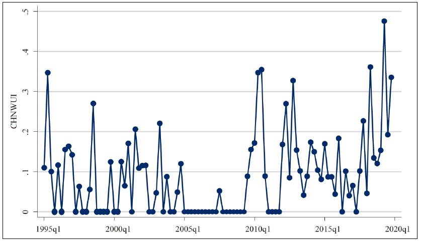
Note: World Uncertainty Index for China from 1995 to 2019
Table 2.
List of Country
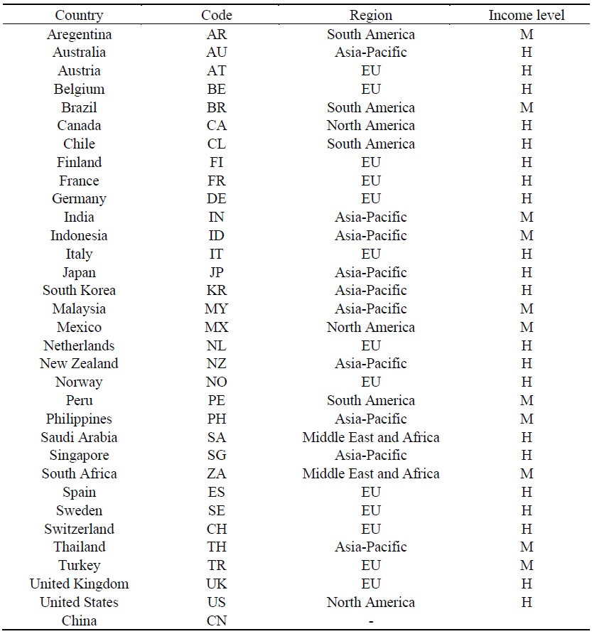
Figure 2.
China and the US: Pre-Financial Crisis vs Post-Financial Crisis
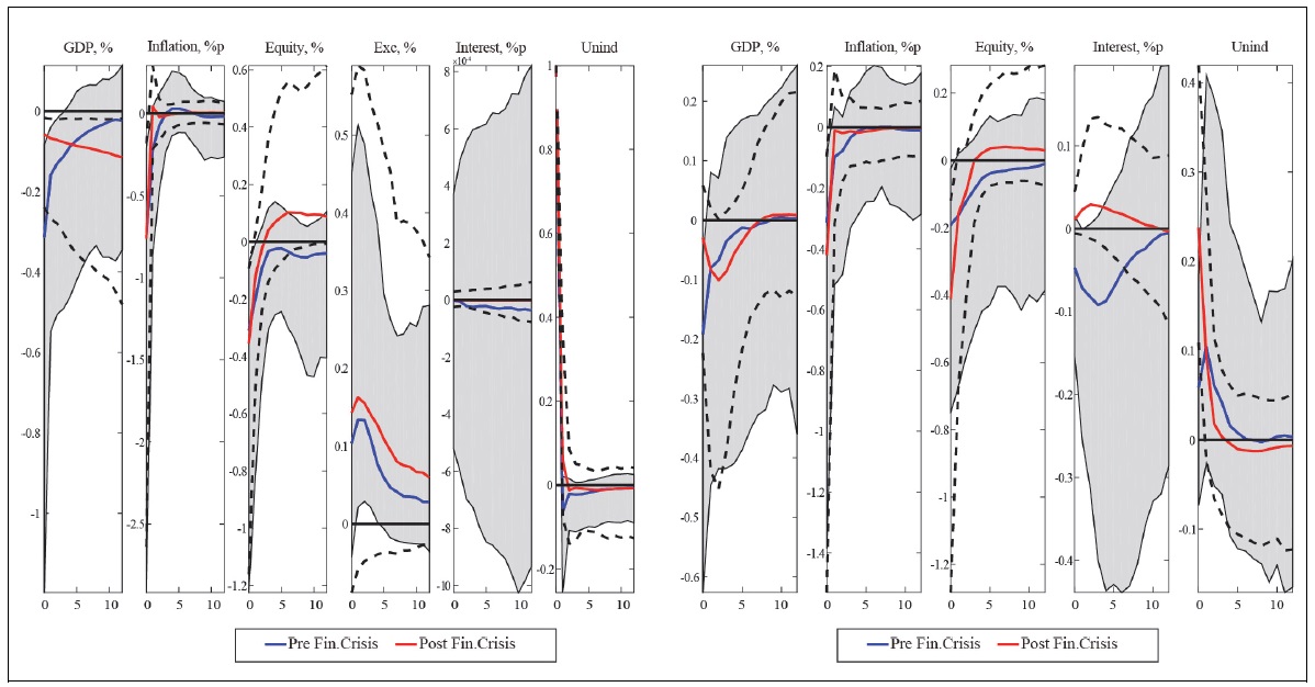
Notes: Left panel depicts China and Right panel depicts the US. Blue line and shaded areas indicate the median responses in the pre-financial crisis and associated 68% confidence bands. Red line and black dotted line indicate the median responses in the post-financial crisis and associated 68% confidence bands.
Figure 3.
China: Time-varying Responses along Time and Horizons
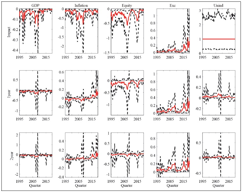
Notes: Red line and black dotted line indicate the median responses and the associated 68% confidence bands. The size of shocks is normalized by one unit increase in China’s uncertainty index.
Figure 4.
U.S.: Time-varying Responses along Time and Horizons
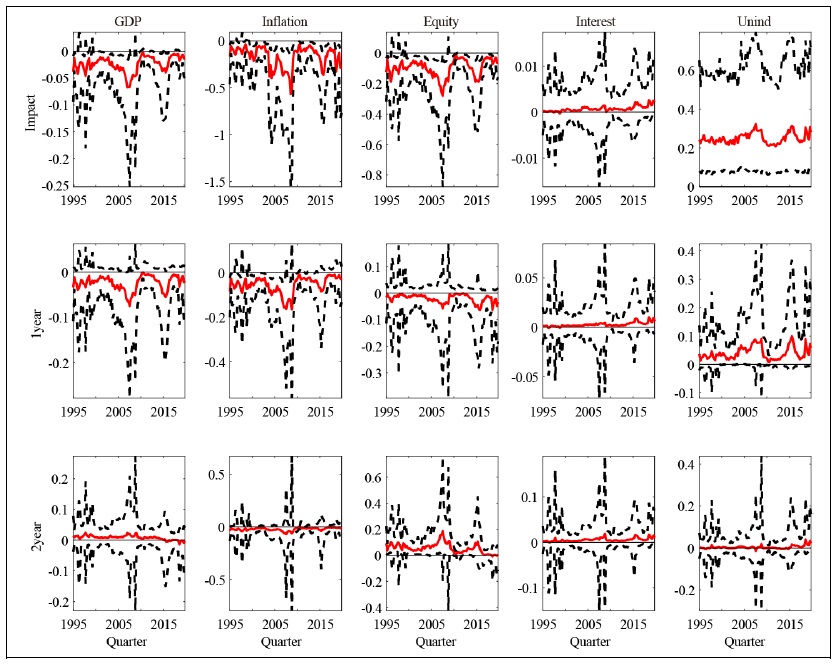
Note: Red line and black dotted line indicate the median responses and associated 68% confidence bands.
Figure 5.
Selected Countries in Europe: Time-varying Responses along Time and Horizons
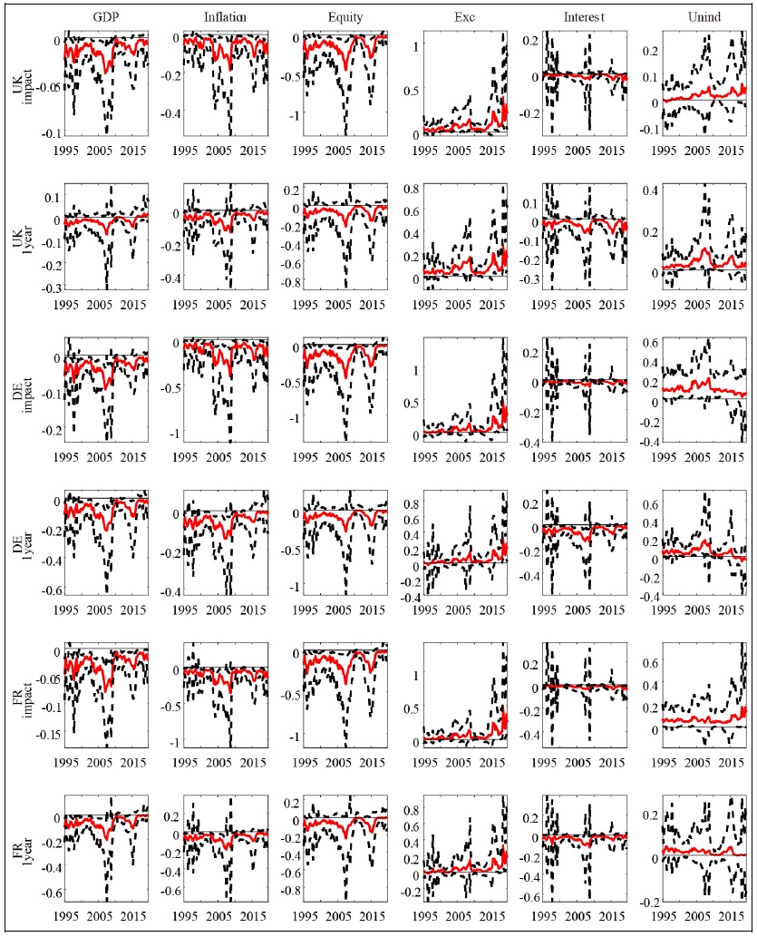
Note: Red line and black dotted line indicate the median responses and associated 68% confidence bands.
Figure 6.
Selected Countries in North and South America: Time-varying Responses along Time and Horizons
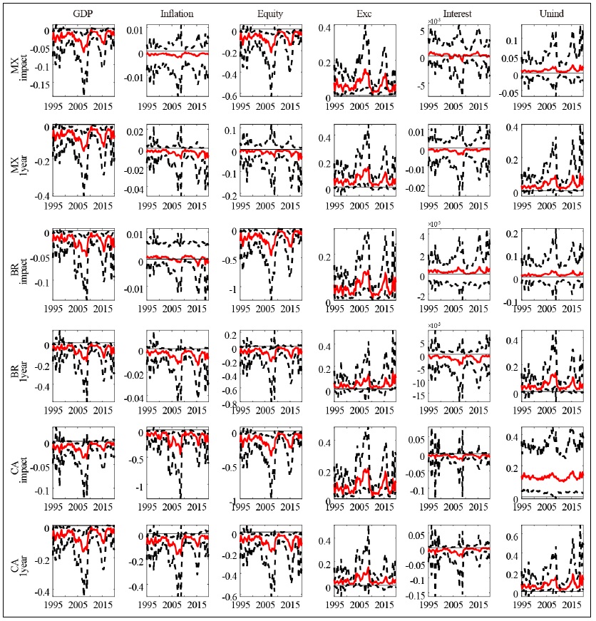
Figure 7.
Selected Countries in Asia: Time-varying Responses along Time and Horizons
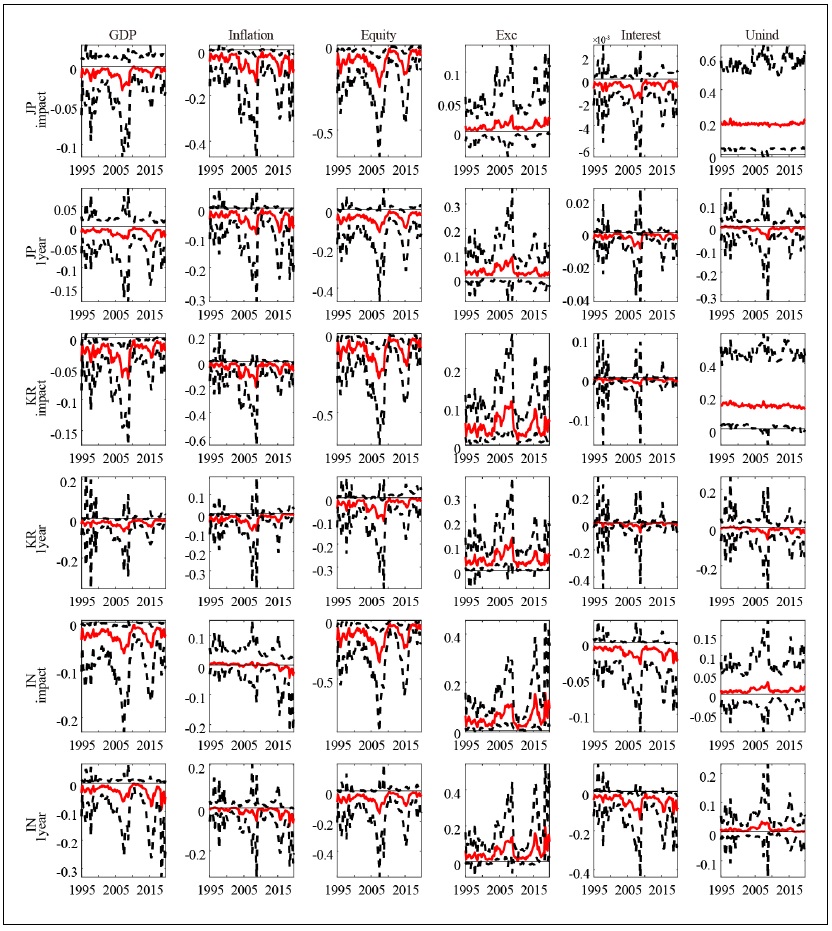
Note: Red line and black dotted line indicate the median responses and the associated 68% confidence bands.
Figure 8.
Distribution of Median Responses on Impact by Countries
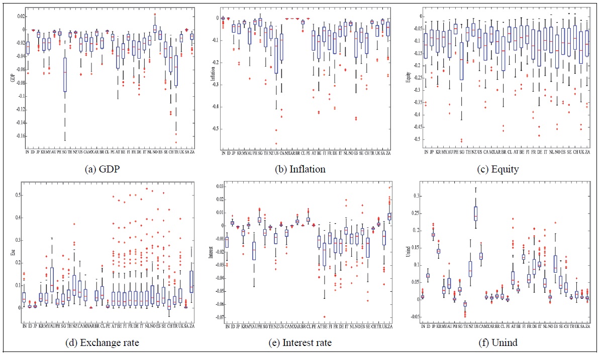
Figure 9.
Geographical Distribution of Min-Max of Median Responses on Impact
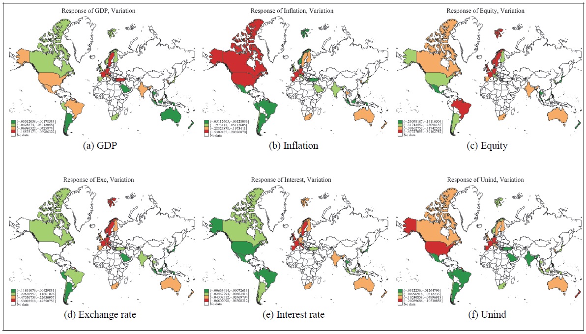
Note: Red means more vulnerable to China’s uncertainty shocks.
Table 3.
Openness, Monetary Policy and Variability of Responses
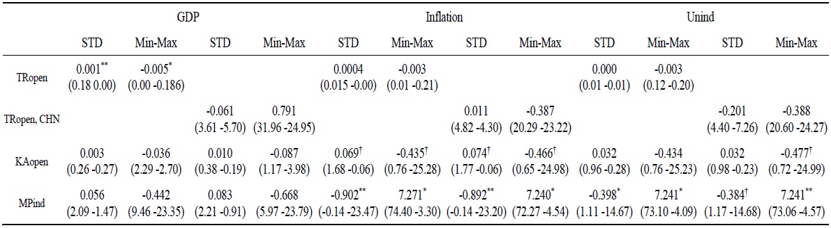
Notes: ∗∗, ∗, †: significant at 95%, 90%, and 68%, respectively. I report median and 95% credible intervals (numbers in parentheses). For the inferences, I use the following 3 steps. First, I compute standard deviation and min-max of responses of GDP, inflation and Unind for each country as dependent variables using each of 1,000 posterior draws from the identified TVP-BGVAR. After those, I obtain total 1,000 number of each dependent variable. Second, I estimate Bayesian regressing model using a Gibbs sampling algorithm, standard normal-inverse gamma prior, and each generated dependent variables. For Gibbs sampling, I generate 11,000 draws and burn-in the first 10,000 draws for each dependent variable. Third, of remaining 1,000 posterior for each dependent variable, I compute the confidence intervals (thus for the inference, I use total 1,000 times 1,000 draws for each dependent variable.).
APPENDIX A: Prior for TVP-BGVAR
In this appendix, I explain prior specification for the TVP-BGVAR. Most specifications are the same as those in Crespo-Cuaresma et al. (2019).
(1)
(2)  I assume that
 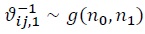 where
where
(3)  where
where
(4)
(5)  with
with
(6)  features non-conjugate gamma prior with
  In the estimation,
APPENDIX B: Estimation Procedures
In this appendix, I explain markov chain monte carlo (MCMC) algorithm for the TVP-BGVAR. The algorithm is the same as that in Crespo-Cuaresma et al. (2019). Note that full history of the time varying elements for time
(1) Step 1: Using the well-known Carter-Kohn procedure,  is sampled.
(2) Step 2: Given  the posterior of
  is independent of the data and follows
(3) Step 3: The posterior of each element of 
(4) Step 4:  is each element of
(5) Step 5: 
(6) Step 6: Log volatilities are sampled using the algorithm proposed by Kastner and Fruhwirth-Schnatter (2014). Other detailed procedures are the same in Crespo-Cuaresma et al. (2019) .
APPENDIX C: Supplement Figures
I compute average responses of high income countries and middle income countries and four regions. I take the simple average of each income group and region using each 1,000 posterior draws from the identified TVP-BGVAR model. Then, I get 1,000 posterior draws for each group. Using those posteriors, I compute the median and the associated 68% credible intervals for each group. Figure 10 and Figure 11 show the results for the income group and regions, respectively.
Appendix Tables & Figures
Figure 10.
Response by Income Level: On Impact
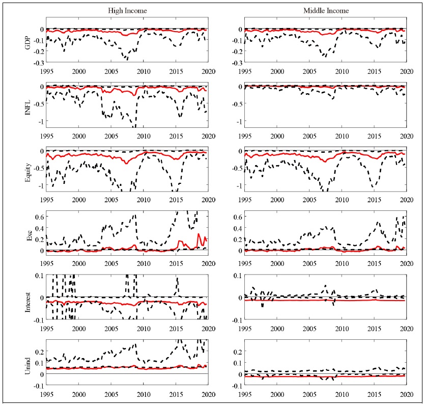
Note: Red line and black dotted line indicate the median responses and the associated 68% confidence bands.
Figure 11.
Response by Regions: On Impact
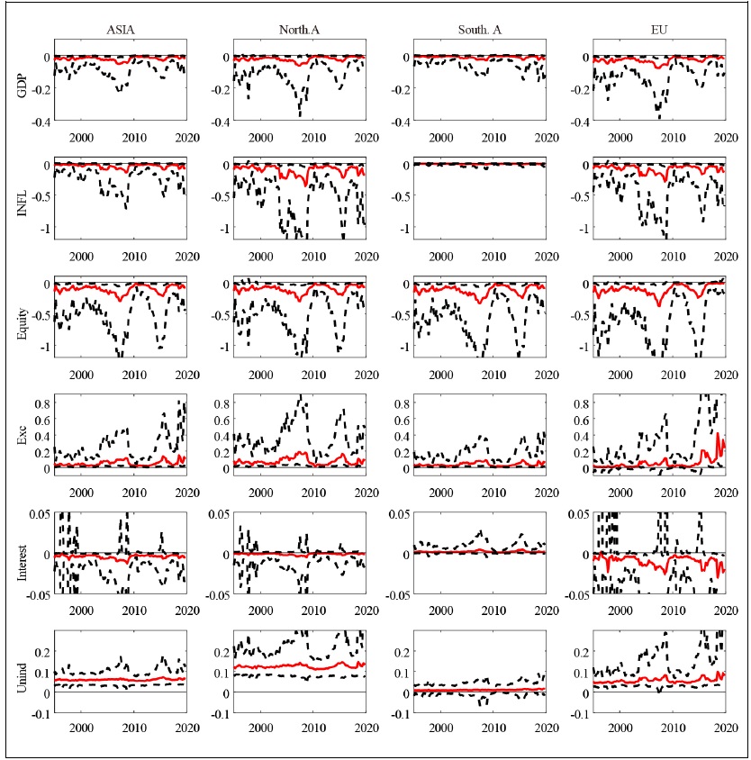
Note: Red line and black dotted line indicate the median responses and the associated 68% confidence bands.
References
- Ahir, H., Bloom, N. and D. Furceri. 2022. “The world uncertainty index.” NBER Working Papers, no. 29763. National Bureau of Economic Research.
-
Aizenman, J., Chinn, M. D. and H. Ito. 2010. “The emerging global financial architecture: Tracing and evaluating new patterns of the trilemma configuration.”
Journal of International Money and Finance , vol. 29, no. 4, pp. 615-641.
-
Baker, S. R., Bloom, N. and S. J. Davis. 2016. “Measuring economic policy uncertainty.”
Quarterly Journal of Economics , vol. 131, no. 4, pp. 1593-1636.
-
Basu, S. and B. Bundick. 2017. “Uncertainty shocks in a model of effective demand.”
Econometrica , vol. 85, no. 3, pp. 937-958.
-
Belke, A. and T. Osowski. 2019. “International effects of euro area versus us policy uncertainty: A favar approach.”
Economic Inquiry , vol. 57, no. 1, pp. 453-481.
-
Bhattarai, S., Chatterjee, A. and W. Y. Park. 2020. “Global spillover effects of us uncertainty.”
Journal of Monetary Economics , vol. 114, pp. 71-89.
-
Bloom, N. 2009. “The impact of uncertainty shocks.”
Econometrica , vol. 77, no. 3, pp. 623-685.
-
Böck, M., Feldkircher, M. and P. L. Siklos. 2021. “International effects of euro area forward guidance.”
Oxford Bulletin of Economics and Statistics , vol. 83, no. 5, pp. 1066-1110.
-
Carrière-Swallow, Y. and L. F. Céspedes. 2013. “The impact of uncertainty shocks in emerging economies.”
Journal of International Economics , vol. 90, no. 2, pp. 316-325.
-
Chen, K., Ren, J. and T. Zha. 2018. “The nexus of monetary policy and shadow banking in china.”
American Economic Review , vol. 108, no. 12, pp. 3891-3936.
-
Chinn, M. D. and H. Ito. 2006. “What matters for financial development? capital controls, institutions, and interactions.”
Journal of Development Economics , vol. 81, no. 1, pp. 163-192.
-
Chudik, A., Mohaddes, K. and M. Raissi. 2021. “Covid-19 fiscal support and its effectiveness.”
Economics Letters , vol. 205.
-
Chudik, A. and M. H. Pesaran. 2016. “Theory and practice of GVAR modelling.”
Journal of Economic Surveys , vol. 30, no. 1, pp. 165-197.
-
Cogley, T. and T. J. Sargent. 2005. “Drifts and volatilities: monetary policies and outcomes in the post WWII US.”
Review of Economic Dynamics , vol. 8, no. 2, pp. 262-302.
-
Crespo-Cuaresma, J., Doppelhofer, G., Feldkircher, M. and F. Huber. 2019. “Spillovers from us monetary policy: evidence from a time varying parameter global vector autoregressive model.”
Journal of the Royal Statistical Society Series A: Statistics in Society , vol. 182, no. 3, pp. 831-861.
- Davis, S. J., Liu, D. and X. S. Sheng. 2019. “Economic policy uncertainty in china since 1949: The view from mainland newspapers.” Paper presented in the Fourth IMFAtlanta Fed Research Workshop on China’s Economy. Atlanta. September 19-20, 2019. Federal Reserve Bank of Atlanta.
-
Dees, S., di Mauro, F., Pesaran, M. H. and L. V. Smith. 2007. “ Exploring the international linkages of the euro area: a global var analysis.”
Journal of Applied Econometrics , vol. 22, no. 1, pp. 1-38.
-
Diebold, F. X. and K. Yılmaz. 2014. “On the network topology of variance decompositions: Measuring the connectedness of financial firms.”
Journal of Econometrics , vol. 182, no. 1, pp. 119-134.
-
Eickmeier, S. and M. Kühnlenz. 2018. “China’s role in global inflation dynamics.”
Macroeconomic Dynamics , vol. 22, no. 2, pp. 225-254.
-
Fernald, J. G., Spiegel, M. M. and E. T. Swanson. 2014. “Monetary policy effectiveness in china: Evidence from a favar model.”
Journal of International Money and Finance , vol. 49, pp. 83-103.
-
Fontaine, I., Razafindravaosolonirina, J. and L. Didier. 2018. “Chinese policy uncertainty shocks and the world macroeconomy: Evidence from STVAR.”
China Economic Review , vol. 51, pp. 1-19.
-
Gambetti, L. and A. Musso. 2017. “Loan supply shocks and the business cycle.”
Journal of Applied Econometrics , vol. 32, no. 4, pp. 764-782.
- Geiger, M. 2008. “Instruments of monetary policy in China and their effectiveness: 1994-2006.” UNCTAD Discussion Papers, no. 187. United Nations Conference on Trade and Development.
-
Han, L., Qi, M. and L. Yin. 2016. “Macroeconomic policy uncertainty shocks on the chinese economy: a GVAR analysis.”
Applied Economics , vol. 48, no. 51, pp. 4907-4921.
-
Huang, Y. and P. Luk. 2020. “Measuring economic policy uncertainty in china.”
China Economic Review , vol. 59.
-
Huang, Z., Tong, C., Qiu, H. and Y. Shen. 2018. “The spillover of macroeconomic uncertainty between the US and China.”
Economics Letters , vol. 171, pp. 123-127.
-
Jiang, Y., Zhu, Z., Tian, G. and H. Nie. 2019. “Determinants of within and cross-country economic policy uncertainty spillovers: Evidence from US and China.”
Finance Research Letters , vol. 31.
-
Jones, P. M. and E. Olson. 2015. “The international effects of us uncertainty.”
International Journal of Finance & Economics , vol. 20, no. 3, pp. 242-252.
-
Kastner, G. and S. Frühwirth-Schnatter. 2014. “Ancillarity-sufficiency interweaving strategy (ASIS) for boosting MCMC estimation of stochastic volatility models.”
Computational Statistics & Data Analysis , vol. 76, pp. 408-423.
-
Kim, W. 2020. “Impacts of RMB devaluation on china’s trade balances: a time-varying svar approach.”
Applied Economics , vol. 52, no. 45, pp. 4952-4966.
-
Klößner, S. and R. Sekkel. 2014. “International spillovers of policy uncertainty.”
Economics Letters , vol. 124, no. 3, pp. 508-512.
-
Lakdawala, A., Moreland, T. and M. Schaffer. 2021. “The international spillover effects of us monetary policy uncertainty.”
Journal of International Economics , vol. 133.
- Lastauskas, P. and A. Nguyen. 2021. “Global impacts of us monetary policy uncertainty shocks.” ECB Working Paper Series, no. 2513. European Central Bank.
-
Leduc, S. and Z. Liu. 2016. “Uncertainty shocks are aggregate demand shocks.”
Journal of Monetary Economics , vol. 82, pp. 20-35.
-
Ludvigson, S. C., Ma, S. and S. Ng. 2021. “Uncertainty and business cycles: exogenous impulse or endogenous response?”
American Economic Journal: Macroeconomics , vol. 13, no. 4, pp. 369-410.
-
Mohaddes, K. and M. Raissi. 2020. “Compilation, revision and updating of the global VAR (GVAR) database, 1979Q2-2019Q4.” August 7.
Mimeo .https://www.econ.cam.ac.uk/people-files/faculty/km418/GVAR%20Database%20(1979Q2-2019Q4).pdf -
Mwase, N., N’Diaye, P. M., Oura, H., Ricka, F., Svirydzenka, K. and Y. S. Zhang. 2016.
Spillovers from China: financial channels . International Monetary Fund. -
Pesaran, M. H., Schuermann, T. and S. M. Weiner. 2004. “Modeling regional interdependencies using a global error-correcting macroeconometric model.”
Journal of Business & Economic Statistics , vol. 22, no. 2, pp. 129-162.
-
Primiceri, G. E. 2005. “Time varying structural vector autoregressions and monetary policy.”
Review of Economic Studies , vol. 72, no. 3, pp. 821-852.
- Redl, C. 2017. “The impact of uncertainty shocks in the United Kingdom.” Staff Working Paper, no. 695. Bank of England.
-
Redl, C. 2020. “Uncertainty matters: evidence from close elections.”
Journal of International Economics , vol. 124.
-
Rubio-Ramirez, J. F., Waggoner, D. F. and T. Zha. 2010. “Structural vector autoregressions: Theory of identification and algorithms for inference.”
Review of Economic Studies , vol. 77, no. 2, pp. 665-696.
- Shu, C. He, D. Wang, H. and J. Dong. 2015. “The influence of chinese and us financial markets on asia-pacific.” Paper presented in the joint conference of Cross-border Financial Linkages: Challenges for Monetary Policy and Financial Stability. Wellington, New Zealand. 23-24 October, 2014.
-
Stock, J. H. 2001. “[Evolving post-World War II US inflation dynamics]: Comment.”
NBER Macroeconomics Annual , vol. 16, pp. 379-387.
-
You, W., Guo, Y., Zhu, H. and Y. Tang. 2017. “Oil price shocks, economic policy uncertainty and industry stock returns in china: Asymmetric effects with quantile regression.”
Energy Economics , vol. 68, pp. 1-18.
-
Zhang, D., Lei, L., Ji, Q. and A. M. Kutan. 2019. “Economic policy uncertainty in the us and china and their impact on the global markets.”
Economic Modelling , vol. 79, pp. 47-56